4
In this chapter, the sections follow the order in which commands and options appear beginning with those found under the File menu and ending with those under the Help menu.
Many of the commands and options that appear under these menus are also accessible by other methods. Consequently, these other methods are also explained.
When spSlab/spBeam is loaded, the program is ready to begin receiving input for a new project. Until you save the file, the data will not have a filename associated with it, and the title bar will display the word spSlab1 or spBeam1 as illustrated here:
•From the File menu, choose New. This clears the screen in preparation for a new project or data entry file and returns the program to its default settings.
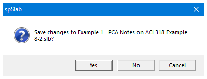
•If existing data on an open project has been changed prior to executing the New command, the program will display the following message box inquiring whether you wish to save the data on the open project or data file before creating a new file:
spSlab allows you to open data files that were saved at an earlier time including files from previous versions of spSlab and spBeam as well as pcaSlab, pcaBeam, or ADOSS. Note that the extension name of an ADOSS .ADS and the extention name of a pcaBeam v1.01 file is .BMS. Both pcaSlab and pcaBeam v1.5x use files with the .SLB extension.
•From the File menu, choose Open and a dialog box will appear.
•All files with the .SLB extension contained in the current drive and directory are displayed in the File Name list box. To view files with a different extension, use the file type drop-down menu to choose a different file extension.
•To open a file that exists in another drive or directory, select the drive or directory you want from the Look in drop-down list.
•From the File Name list box, select the file to be opened, or simply type its name in the text box.
•Choose the OK button.
•Alternatively, an input file can be opened by spSlab if the file is drag-and-dropped onto the program window or if the file pathname is provided as a command line parameter when invoking spSlab from the command prompt.
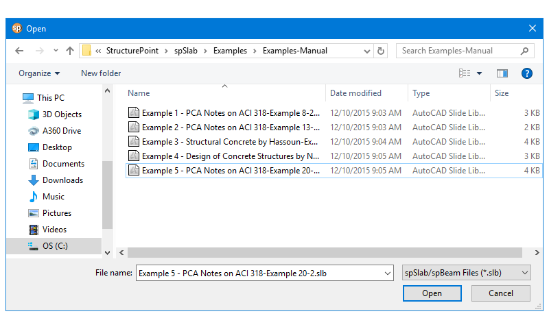
Figure 4-1 Open Dialog Box
spSlab files are saved in a binary format with .SLB extensions.
4.4.1Save the data with the same file name
•At any time while editing a data file that has previously been saved under a file name, choose File and Save to save the changes under the same file name, overwriting the old file. From the File menu, select the Save command before giving the data file a name displays the Save As dialog box.
4.4.2Change the format or rename the file
•From the File menu, select Save As, and a dialog box will appear.
•All files with. SLB extensions contained in the current drive and directory are displayed in the File Name list box.
•To save the file to a drive or directory other than the default, select a different drive or directory from the Save In drop-down list.
•Choose OK button
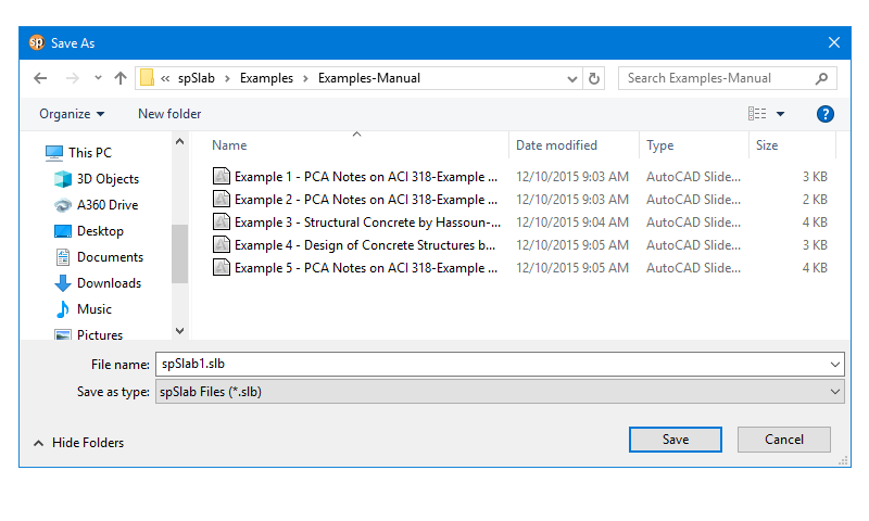
Figure 4-2 Save As Dialog Box
4.5Most Recently Used Files (MRU)
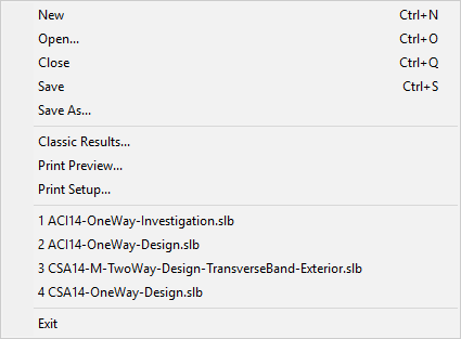
Figure 4-3 Most Recently Used File List (MRU)
The Most Recently Used Files (MRU) list shows the four data files that were opened most recently. Selecting a data file from this list makes it easier and faster to open the file. The list is empty when the program is executed for the first time.
4.6Specifying Model Data (Menu Input)
The Data Input Wizard is designed to make the inputting process easier. By selecting the Data Input Wizard from Input menu or selecting  from the tool bar, a logical sequence of dialog boxes will automatically be displayed allowing you to enter data for your floor system.
4.7Defining General Information
The General Information command allows you to enter labels, design code, reinforcement database, run mode, and the frame information needed by spSlab to proceed with the input process. You must choose this command before doing any further inputting since this command affects the availability of the commands in the Input menu.
To enter general information:
•Select the General Information command from the Input menu or click the  button from the tool bar. The dialog box of Figure 4-4 will appear.
•Enter the project name, frame name, and engineer name in the Label frame box.
•Select the building standard you want your floor system to be designed to (ACI 318-14, ACI318M-14, ACI 318-11, ACI 318M-11, ACI 318-08, ACI 318M-08, ACI 318-05, ACI 318M-05, ACI 318-02, ACI 318M-02, ACI 318-99, ACI 318M-99, CSA A23.3-14, CSA A23.3-14E, CSA A23.3-04, CSA A23.3-04E, CSA A23.3-94, CSA A23.3-94E) from the Option frame box.
a)  b)
b) 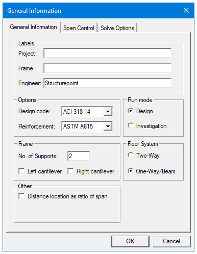
Figure 4-4 General Information dialog box (a) two-way system (b) beam and one-way system
•Select the Design or Investigation from the Run mode frame box.
•In the Frame box, enter the Number of supports of the frame. The default number of supports is 2. The minimum and maximum number of spans is 1 and 20 spans, respectively. Therefore the minimum number of supports is 2 and the maximum number of supports is 21.
•Check the Left cantilever and/or Right cantilever check boxes if left cantilever and/or right cantilever exist in the frame respectively.
•In the Floor System frame box, select Two-Way or Beams/one-way slab option.
•Select None, Longitudinal, or Transverse in Slab Band box if a two-way floor system is selected for the CSA A23.3-14/04 design code.
•Check the Distance location as ratio of span if the locations of loads need to be entered as a ratio of the length of a span.
•Press Ok button to exit the dialog box and allow spSlab to use the new data. If using the Auto Input, click the Next button to the next dialog box.
The Solve Options command allows you to select options and specify parameters that affect the analysis and design results. Changing these settings involves engineering judgment and it has to be done cautiously. To take effect, this command must be used prior to the Execute command. The set of parameters is different for two-way and one-way systems.
To specify solve options for two-way systems:
•Enter the live load pattern ratio.
•Check Compression Reinforcement checkbox if it is to be considered when needed.
•Check User Slab Strip Width to enable manual input of column strip width. The default values are calculated according to design code selected. The validity of the assumptions when entering user defined values are to be decided by the Designer.
•Check User Distribution Factors to enable manual input of moment distribution factors. The default values are calculated according to design code selected. The validity of the assumptions when entering user defined values are to be decided by the Designer.
•Check Decremental reinforcement Design to use alternative reinforcement design algorithm.
•Check Combined M-V-T Reinf. Design to proportion longitudinal reinforcement for combined action of flexure, shear, and torsion. This option is available only when CSA A23.3-14 or CSA A23.3-04 are selected.
•Check One-Way Shear In Drop Panels to include drop panel cross-section in slab one-way shear capacity calculations in support locations.
•Check Distribute Shear to Slab Strips to distribute slab one-way shear between column and middle strips in proportion to moment distribution factors.
•Check Beam T-Section Design to include portions of slab as flanges in beam cross-section for reinforcement design.
•Check Long. Bm. Supt. Design to include cross-section of longitudinal beam in reinforcement design for unbalanced moments over supports. This feature can be useful for slabs having wide longitudinal beams. When used together with User Distribution Factors, it can produce solutions consistent with the solutions for models with longitudinal slab bands for CSA A23.3-14/04 code.
•Check Trans. Bm. Supt. Design to include cross-section of transverse beam in reinforcement design for negative moments and unbalanced moments over supports. This feature is useful for slabs having wide transverse beams. When used together with User Distribution Factors, it can produce solutions consistent with the solutions for systems with transverse slab bands for CSA A23.3-14/04 code.
•Enter the multiplier that defines the distance between a column face and a free edge of a slab, within which a segment of punching shear critical section is to be ignored.
•Select whether circular critical section around circular supports is to be used or traditional equivalent rectangular critical section.
•Choose if Gross (uncracked) or Effective (cracked) sections are to be considered in the deflection calculations.
•Choose if in the case of a section with flanges in the negative moment region, only the web (Rectangular Section) or the whole section (T-Section) is to be used to calculate the gross moment of inertia (Ig) and the cracking moment.
•Check Calculate long-term deflections checkbox if you want the program to calculate long-term deflections. Provide the duration of load in months and the percentage of the live load which is considered as sustained load.
ACI
a) 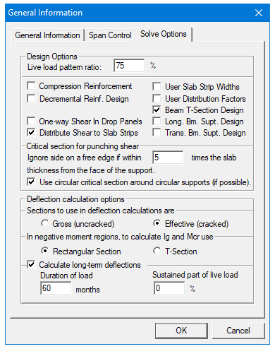 b)
b) 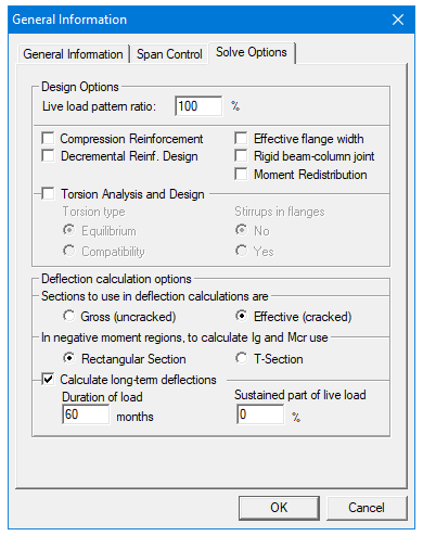
CSA
c) 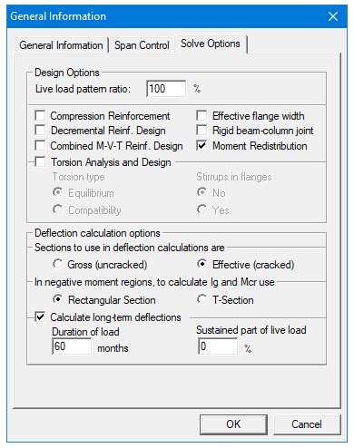 d)
d) 
Figure 4-5 Solve Option (a, d) two-way system (b,c) beam and one-way system
To specify solve options for beams/one-way slab systems:
•Enter the live load pattern ratio. The default value for beams/one-way slab systems is 100%.
•Check Compression Reinforcement checkbox if it is to be considered when needed.
•Check Decremental reinforcement Design to use alternative reinforcement design algorithm.
•Check Combined M-V-T Reinf. Design to proportion longitudinal reinforcement for combined action of flexure, shear, and torsion. This option is available only when CSA A23.3-14 or CSA A23.3-04 are selected.
•Check Effective flange width if instead of the full flange width only the effective flange width is to be considered in the flexural design.
•Check Rigid beam-column joint to consider beam-column joint as rigid.
•Check Torsion analysis and design if they are to be included in the solution. This option has to be checked for the Torsion type and Stirrups in flanges options to be enabled. Also torsional loads will only be available in the Type combo box of the Span Loads dialog box if this option is checked.
•Check Moment Redistribution checkbox if it is to be considered in the analysis. This option has to be checked for the Moment Redistribution tab to be available in the Support Data dialog box.
•If torsion analysis and design is checked then select if Equilibrium or Compatibility torsion is to be considered and if for sections with flanges Stirrups in flanges can be considered.
•Choose if Gross (uncracked) or Effective (cracked) sections are to be considered in the deflection calculations.
•Choose if in the case of a section with flanges in the negative moment region, only the web (Rectangular Section) or the whole section (T-Section) is to be used to calculate the gross moment of inertia (Ig) and the cracking moment.
•Check Calculate long-term deflections checkbox if you want the program to calculate long-term deflections. Provide the duration of load in months and the percentage of the live load which is considered as sustained load.
The Span Control tab allows you to perform different operations on the spans that your system consists of. These operations include inserting new spans with default parameters, creating new spans by copying existing spans, moving spans to change span sequence, and deleting spans. The result of an operation depends on the span selected as well an on the selected support. Spans can be selected using the Span Control List and columns using the Support Selection radio buttons.
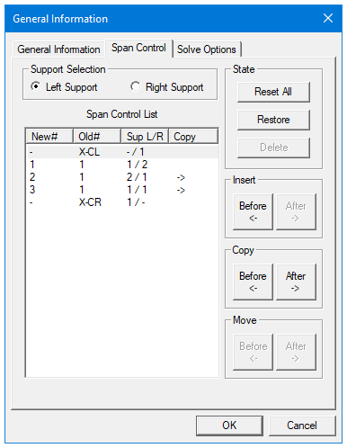
Figure 4-6 Span control tab
Additionally before the Span Control window is closed all changes made to the spans can be revoked using the Reset All button. The Restore button can be used to bring back a span removed using the Delete button.
To insert a new span with default dimensions:
•In the Span Control List select the span next to which you want to insert a new span.
•Select whether the Left Support or the Right Support of the newly created span will be inserted.
•Press Insert Before button to insert the new span left to the selected span or Insert After button to insert the new span on the right side of the currently selected span.
•Examples of the insert operations are presented in Figure 4-7. Assuming that Span 2 is always selected the resulting systems will depend on whether Insert After or Insert Before was used and whether Left Column or Right Column was selected. Newly inserted span and column are denoted with an “x”.
To copy a span:
•In the Span Control List select the span you want to copy.
•Select whether the Left Support or the Right Support of the copied span will be copied with the span.
•Press Insert Before button to place the copied span left to the selected span or Insert After button to place the copied span on the right side of the currently selected span.
•Examples of the insert operations are presented in Figure 4-8. Assuming that Span 2 is always selected the resulting systems will depend on whether Copy After or Copy Before was used and whether Left Column or Right Column was selected. Newly created span and column are denoted with the prime sign.
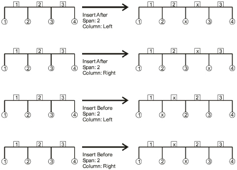
Figure 4-7 Inserting a new span using Span Control
To move a span:
•In the Span Control List select the span you want to move.
•Select whether the Left Support or the Right Support of the moved span will be moved with the span.
•Press Move Before button to move the span to the left or Move After button to move the span to the right side.
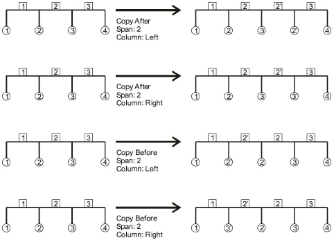
Figure 4-8 Copying a span using Span Control
Examples of the move operations are presented in Figure 4-9. Assuming that Span 2 is always selected the resulting systems will depend on whether Move After or Move Before was used and whether Left Column or Right Column was selected.
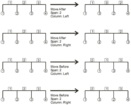
Figure 4-9 Moving a span using Span Control
To delete a span:
•In the Span Control List select the span you want to delete.
•Select whether the Left Support or the Right Support of the deleted span will be removed with the span.
•Press the Delete button to delete the selected span.
Examples of the delete operations are presented in Figure 4-10. Assuming that Span 2 is always selected the resulting systems will depend on whether Left Column or Right Column was selected.
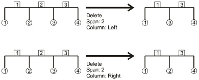
Figure 4-10 Deleting a span using Span Control
4.7.3Defining Material Properties
The Material Properties command from the Input menu allows you to input material properties of the concrete and the reinforcement. There are two tabs in this dialog box. One is for concrete and the other is for reinforcing steel. This command must be executed in order to perform a design of the floor system. Use the tab key to get to each edit box then type in your values, or use your mouse and click directly on the desired tab and box, then type in your values. Refer to "Material Properties" for a detailed explanation of the default values.
To define material properties:
•Select the Material Properties command from the Input menu or click the  button on the tool bar. The dialog box of Figure 4-11 will appear.
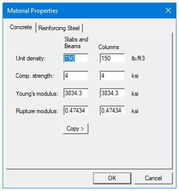
Figure 4-11 Concrete Properties dialog box
•Click the Concrete tab and enter the concrete density for the following members: Slabs, Beams, and Columns.
•Enter the concrete compressive strength. By entering a value for the compressive strength, values for Young’s modulus and rupture modulus will automatically be computed for the slabs, beams, and columns. Young’s modulus and rupture modulus will automatically be shown in the corresponding text boxes.
•If you have values for the rupture modulus, fr, enter the values in the text boxes for the slabs, beams, and columns. Default values are computed based on  . These values will be used for deflection analysis. A large value for the rupture modulus will produce a deflection analysis based on gross, non-cracked, sections. The CSA A23.3 standard requires1 that for the calculation of deflections half the value of rupture modulus be used. spSlab defaults to this value of the rupture modulus for the slab (both one-way and two-way) and beam concrete in CSA A23.3-14/04 design runs and for two-way slabs in CSA A23.3-94 design runs. For beams and one-way slabs per CSA A23.3-94, however, the full value of rapture modulus has to be used and the program will provide it as default in this case. It is strongly recommended, however, that the user verifies what value of fr is actually entered in the program since the default value can be inadvertently overwritten or carried over from a previous run.
•If precast concrete is used, check Precast Concrete checkbox.
•Click the Reinforcing Steel tab as shown in Figure 4-12.
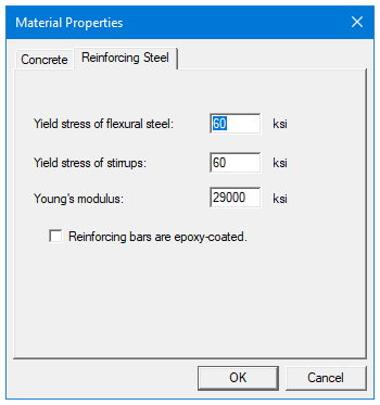
Figure 4-12 Reinforcing Steel Properties dialog box
•Enter the yield stress of flexure steel.
•Enter the yield stress of stirrups.
•Enter the Young’s modulus for flexural steel and stirrups.
•Select whether the main reinforcement is epoxy-coated by clicking the left mouse button on the box or tabbing to the box and pressing the SPACE BAR. This selection affects development lengths.
•Press Ok button to exit the dialog box so that spSlab will use these material properties. If using the Auto Input, click the Next button to the next dialog box.
The Spans command from the Input menu is available for all floor systems. Span numbers, which are determined from the number of supports entered in the General Information box, are automatically filled into the Span drop-down list in the Span Data dialog box.
To input slab geometry:
1.Select the Spans command from the Input menu or click the  button on the tool bar. Click the left mouse button on the Slabs tab. The dialog box of Figure 4-13 will appear.
2.Select the number of the span, for which dimensions will be entered, from the Span drop-down list.
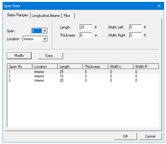
Figure 4-13 Defining the slabs dialog box
3.Select the span location from the Location drop-down list. Three types of locations are available: Interior, Exterior Left, and Exterior Right. The "left" and "right" are defined as you look along the direction of analysis. If a span has design strips on both sides it should be an "Interior" span. If a span has only a left design strip, it should be an "Exterior Right" span. If a span has only a right design strip, it should be an "Exterior Left" span.
4.Enter the slab thickness of the span.
5.Enter the span length from column centerline to column centerline or edge to column centerline for the two cantilever spans in the Length edit box. If the program detects a cantilever span length less than one-half the column dimension in the direction of analysis, an error message will pop up when the frame is analyzed. If a partial load is affected by the span length, a message warns the user of this condition.
6.Enter the span design width in the transverse direction of analysis on the left and right side of the column (see Figure 4-14). These distances are usually one-half the distance to the next transverse column or edge of the slab for exterior spans. The left and right designations are arbitrary. Both interior and exterior spans may be used in a design strip. An exterior width will automatically be designated by spSlab by entering a width value less than or equal to the transverse column dimension. Exterior sides do not contribute to the attached torsional stiffness, although they do contribute to loading. spSlab will use the total width entered for weight and superimposed loading but will use code allowed dimensions for flange width and stiffness computations.
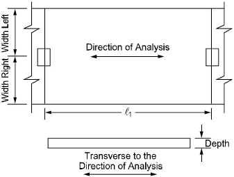
Figure 4-14 Required Slab Dimensions
7.Press the Modify button to update the slab geometry.
8.Repeat steps 2 through 7 until all the spans have been updated. You can use the Copy button as a shortcut.
9.Press Ok button to exit the dialog box and allow spSlab to use the updated slab geometry.
4.7.5Defining Longitudinal Beams
Longitudinal beam dimensions are required for the beam-supported slab. Span numbers, which are determined from the number of supports entered in the General Information box, are automatically filled into the Span drop-down list.
To input longitudinal beam geometry:
1.Select the Spans command from the Input menu or click the  button on the tool bar. Select Longitudinal Beams tab from the Span Data dialog box. The dialog box of Figure 4-15 will appear.
2.Select the span number from the Span drop-down list.
3.Enter the width of the longitudinal beam (Figure 4-16).
4.Enter the depth of the longitudinal beam which is taken from the top of the slab to the bottom of the beam (Figure 4-16).
5.If required, enter the offset which is measured from the joint centerline, positive to the right, and negative to the left of the joint (Figure 4-16)
6.Press the Modify button to update the longitudinal beam geometry.
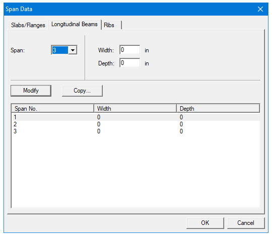
Figure 4-15 Longitudinal Beam Geometry dialog box
7.Repeat steps 2 through 6 until all the beams have been updated. You can use the Copy button as a shortcut.
8.Press Ok button to exit the dialog box so that spSlab will use the new beam geometry.
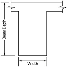
Figure 4-16 Required Longitudinal Beam Dimensions
For joist systems, you must define the rib geometry. The ribs are assumed to be the same throughout the strip.
To enter rib geometry:
•Select the Spans command from the Input menu or click the  button on the tool bar. Click the left mouse button on the Ribs tab. The dialog box of Figure 4-17 will appear.
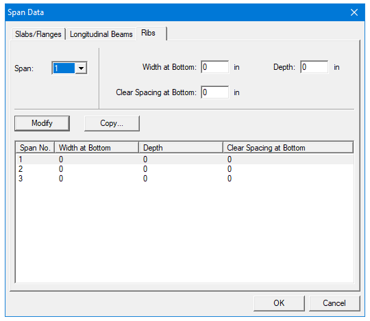
Figure 4-17 Ribs Geometry dialog box
•Select the span number from the Span drop-down list.
•Enter the spacing between ribs at the bottom for clear rib spacing (see Figure 4-18).
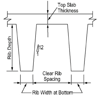
Figure 4-18 Required Rib Dimensions
•Enter the width at the bottom for rib width (see Figure 4-18).
•Enter the depth of the rib below the slab for Rib depth (see Figure 4-18).
•Press Ok button to exit the dialog box so that spSlab can use the rib geometry.
4.7.7Defining Longitudinal Slab Bands
This command is only available for two way floor systems when Slab Bands | Longitudinal option is selected under the General Information dialog box, (CSA A23.3-14/04 only).
The Longitudinal Slab Bands property page (Figure 4-19) allows inputting the width, depth, and offset (eccentricity) of longitudinal slab bands in each span. The procedure is identical to the described earlier input of dimensions of longitudinal beams. It is not required to input bands for every span. Spans where slab bands are not defined are modeled similar to regular two-way systems. Longitudinal slab bands can also be extended to adjacent spans using drop panels.
To input geometry for longitudinal slab band:
1.Select the Spans command from the Input menu or click the  button on the tool bar. Click the left mouse button on the Longitudinal Bands tab. The dialog box of Figure 4-19 will appear.
2.Select the span number from the Span drop-down list.
3.Enter the width of the longitudinal slab band.
4.Enter the depth of the longitudinal slab band from the top of the slab.
5.If required, enter the offset which is measured from the joint centerline, positive to the right, and negative to the left of the joint (See Figure 4-15)
6.Press the Modify button to update the longitudinal slab band geometry.
7.Repeat steps 2 through 6 until all the slab bands have been updated. You can use the Copy button as a shortcut.
8.Press Ok button to exit the dialog box longitudinal slab bands can either be continuous (at every span) or be discontinuous (at a single span or in successive spans). However, discontinuous Longitudinal bands are required to be capped by a half drop panel at the discontinued support.
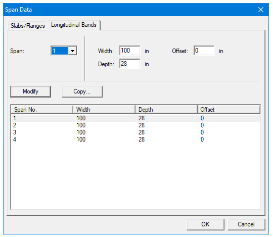
Figure 4-19 Longitudinal Slab Bands Geometry dialog box
4.7.8User Defined Column Strip Widths
User has the ability to manually adjust column strip widths if the two-way floor system option is selected in Solve Options. In this case the Slab/Flanges property page (Figure 4-20) will contain additional field for inputting column strip width. The values of middle and beam strip widths are recalculated internally.
To manually adjust column strip widths:
•Enable check box User Slab Strip Width under Solve Options dialog window.
•Follow the procedure described in section Defining Slabs/Flanges.
•Enter additional values of column strip width for each span.
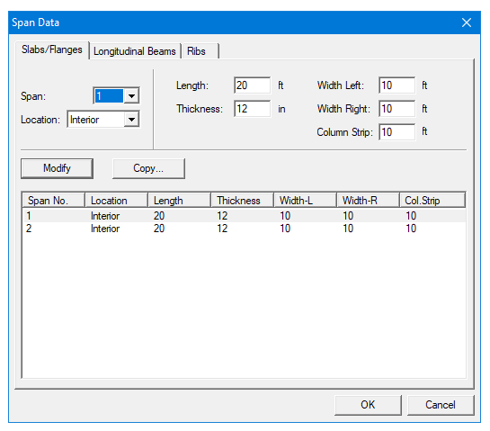
Figure 4-20 User Defined Column Strip Widths
4.7.9User Defined Moment Distribution Factors
User has the ability to manually adjust moment distribution factors if the two-way floor system option is selected in Solve Options. In such case the Moment Distribution property page (Figure 4-21) will become available under Span Data dialog window. This dialog contains fields for inputting distribution factors in column and beam strips. The distribution factors for middle strip are recalculated internally.
To input Moment Distribution Factors:
1.Enable check box User Distribution Factors under Solve Options dialog window.
2.Select the Spans command from the Input menu or click the  button on the tool bar. Click the left mouse button on the Moment Distribution tab. The dialog box of Figure 4-22 will appear.
3.Select the number of the span, for which values will be entered, from the Span drop-down list.
4.Enter moment distribution values in edit boxes.
5.Press the Modify button to update the slab geometry.
6.Repeat steps 2 through 5 until all the spans have been updated. You can use the Copy button as a shortcut.
7.Press Ok button to exit the dialog box.
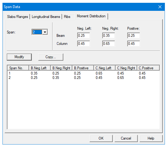
Figure 4-21 User Defined Moment Distribution Factors
Column data is optional. If no column is specified at the joints the joint is assumed hinged. You will be allowed to enter column dimensions above and below.
To input column/capital geometry:
1.Select the Supports command from the Input menu or click the  button on the tool bar. The dialog box of Figure 4-22 will appear. Click on the Columns tab.
2.Enter stiffness share of the column which determines the percentage of the column stiffness used in the analysis. When the percentage lies between zero and 100%, the joint stiffness contribution by the column is multiplied by that percentage. Zero stiffness share indicates a pin support. Value of 999 indicates a support with fully fixed rotation. The default value is 100%, i.e. the actual column stiffness.
3.Enter the column height above, which is the distance from the top of the design floor to the top of the floor above (see Figure 4-23). spSlab obtains the clear column height above by subtracting the average slab depth from the height given. Only the slab is considered for the floor system above. A zero dimension for the column heights above and below will create a pin condition.
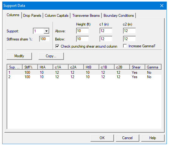
Figure 4-22 Column Geometry dialog box
4.Enter the column height below, which is the distance from the design floor to the top of the floor below (see Figure 4-23). To obtain a clear column height below, the slab/drop/beam depth is subtracted from the height given. A zero dimension for the column heights above and below will create a pin condition.
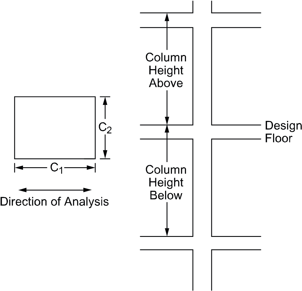
Figure 4-23 Required Column Dimensions
5.Enter a value for c1, the column dimension in the direction of analysis (see Figure 4-23).
6.Enter a value for c2, the column dimension perpendicular to the direction of analysis (see Figure 4-23). Round columns are specified with a zero input for c2; c1 is then taken as the diameter.
7.Select whether spSlab should compute punching shear around column and then ensure the preferred solve option for punching shear perimeter is selected in general information window.
8.Select whether spSlab should compute increased value of gf factor and corresponding decreased gv factor (for ACI code only).
9.Press the Modify button to update the column geometry.
10.Repeat steps 2 through 9 until all the columns and capitals have been updated. You can use the Copy button as a shortcut.
11.Press Ok button to exit the dialog box so that spSlab will use the new data.
Drops are available for the flat slab or waffle slab systems and can be defined at all the support locations. The drop length and width dimensions are computed by spSlab, based on slab span dimensions, when the "Standard" is selected in the Type drop-down list.
To input drop geometry:
1.Select the Supports command from the Input Menu or click the  button then click on the Drop Panels tab. The dialog box of Figure 4-24 will appear.
2.Select whether spSlab should compute the drop dimensions or the dimensions will be user specified. If spSlab is to compute the dimensions, the "Standard" option should be selected from the Type drop-down list and then only the drop depth will be available. When the "Standard drop" option is selected spSlab will calculate drop panel dimensions in accordance with ACI 318 Clause 13.3.7. Similar requirements contained in previous editions of the CSA A23.3 Standard have been removed from the 1994 edition. As a result, the ACI minimum specifications for drop panels are also used in CSA A23.3 runs when the "Standard Drops" option is selected. If you would like to specify drop dimensions other than those computed by spSlab, you must select "User-defined" from the Type drop-down list.
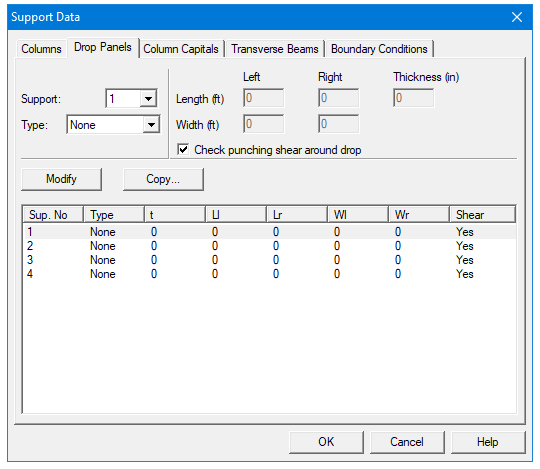
Figure 4-24 Drop Panel Geometry dialog box
3.Enter the dimension in the direction of analysis from the column centerline to the edge of the drop left of the column (see Figure 4-25). If this is a standard drop, this dimension will not be available and the length left is set equal to the slab span length left/6 for interior columns or the left cantilever length for the first column.
4.Enter the width dimension in the transverse direction (see Figure 4-25). If this is a standard drop, this dimension will not be available and the width is set equal to slab width/3.
5.In order for spSlab to recognize drops, drop depths are required for the flat slab systems even if Standard Drop is selected. Enter the depth of the drop from the span with the smaller slab depth (see Figure 4-25). For waffle slab systems, the depth is automatically assumed to be equal to the rib depth below the slab and is not displayed. A value entered will be considered to exist below the rib depth during calculations.
6.Select whether spSlab should compute punching shear around drop panel.
7.Press the Modify button to update the drop geometry.
8.Repeat steps 2 through 6 until all the drop dimensions have been updated. You can use the Copy button as a shortcut.
9.Press Ok button to exit the dialog box so that spSlab will use the new drop geometry
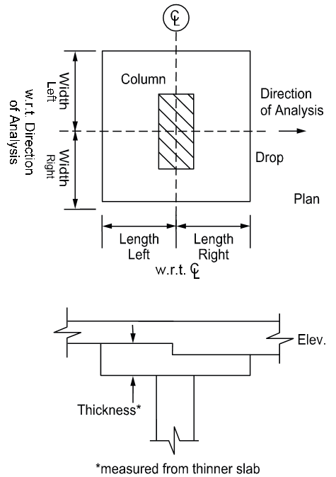
Figure 4-25 Required Drop Panel Dimensions
4.7.12Defining Column Capitals
To input column capital geometry:
•Select the Supports command from the Input menu or click the  button on the tool bar. Click left mouse button on the Column Capitals tab to activate it. The dialog box of Figure 4-26 will appear.
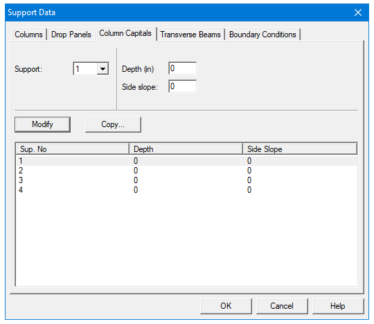
Figure 4-26 Capital Dimensions
•Select the support number from the Support drop-down list.
•Enter the capital depth which is the distance from the bottom of the soffit (slab, drop, or beam), to the bottom of the capital.
•Enter the capital side slope which is the rate of depth to extension of the capital and it must be greater than 1 and smaller than 50 (see Figure 4-27).
•For circular column capitals, ensure the preferred solve option for punching shear perimeter is selected.
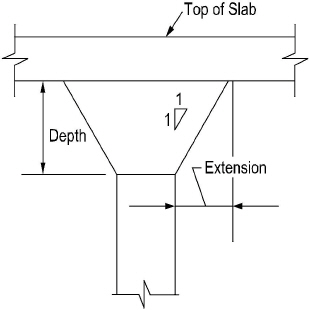
Figure 4-27 Required Capital Dimensions
4.7.13Defining Transverse Beams
This command is only available for two way floor systems when Slab Bands | Transverse option is selected under the General Information dialog box, (CSA A23.3-14/04 only).
The Transverse Beam command allows you to input the width, depth, and offset (eccentricity) of transverse beams at each column. This command is optional.
To input transverse beam geometry:
1.Select the Support command from the Input menu. Select Transverse Beams tab from the Support Data dialog box. The dialog box of Figure 4-28 will appear.
2.Enter the width of the transverse beam (see Figure 4-29)
3.Enter the depth of the transverse beam which is taken from the top of the slab to the bottom of the beam (see Figure 4-29)
4.If required, enter the offset, which is measured from the joint centerline, positive to the right, and negative to the left of the joint (See Figure4-29).
5.Press the Modify button to update the transverse beam dimensions.
6.Repeat steps 2 through 5 until all the beams have been updated. You can use the Copy button as a shortcut (see "Entering the Structure Geometry" earlier in this chapter for help on the Copy button).
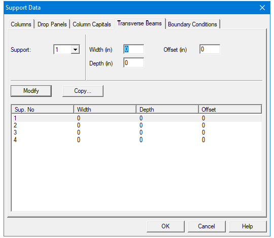
Figure 4-28 Transverse Beam Geometry dialog box
7.Press Ok button to exit the dialog box so that spSlab will use the new beam geometry.
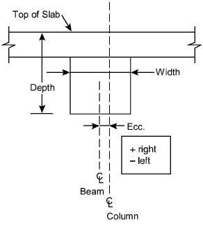
Figure 4-29 Required Transverse Beam Dimensions
4.7.14Defining Transverse Slab Bands
The Transverse Slab Bands property page (Figure 4-30) allows inputting the width, depth, and offset (eccentricity) of transverse bands at each column. It is not required to input bands for every support. Supports where slab bands are not defined are modeled similar to regular two-way systems.
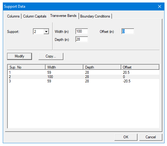
Figure 4-30 Transverse Slab Band Geometry dialog box
To input transverse slab band geometry:
1.Select the Support command from the Input menu. Select Transverse Slab Bands tab from the Support Data dialog box. The dialog box of Figure 4-30 will appear.
2.Enter the width of the transverse slab band (see Figure 4-30)
3.Enter the depth of the transverse slab band which is taken from the top of the slab to the bottom of the slab band (see Figure 4-30).
4.If required, enter the offset, which is measured from the joint centerline, positive to the right, and negative to the left of the joint (See Figure 4-30).
5.Press the Modify button to update the transverse slab band dimensions.
6.Repeat steps 2 through 5 until all the beams have been updated. You can use the Copy button as a shortcut (see "Entering the Structure Geometry" earlier in this chapter for help on the Copy button).
7.Press Ok button to exit the dialog box so that spSlab will use the new band geometry.
4.7.15Defining Boundary Conditions
By default spSlab assumes that column-slab/beam joints can only rotate and that they do not undergo any translational displacements. Rotation of a joint is affected by the stiffness of elements it connects i.e. slabs/beams, transverse beams, and columns. Columns are assumed by default to be fixed at their far ends as shown in Figure 2-6. These default assumptions can be altered using the Boundary Conditions command.
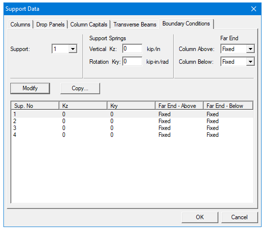
Figure 4-31 Boundary Conditions dialog box
By specifying vertical spring support constant with Kz value other than 0, you can allow the joint to displace vertically. This movement is then controlled by the stiffness of the spring Kz in addition to the stiffness of the column below. The column above is assumed not to constrain the vertical movement of the joint. Additional rotational spring support can be applied to the joint by specifying the value of Kry. Also the far end column conditions can be selected as either fixed or pinned as shown in Figure 4-32(b). All elements controlling the displacements of a joint are shown in Figure 4-32(a).
a)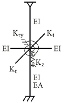 b)
b)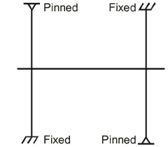
Figure 4-32 (a) Elements controlling joint displacement (b) Far End Column Boundary Conditions
To input boundary conditions:
1.Select the Support command from the Input menu. Select Boundary Conditions tab from the Support Data dialog box. The dialog box of Figure 4-31 will appear.
2.Select support number
3.Enter value of Kz to allow vertical displacement of the support and to add translational spring support (see Figure 4-32(a))
4.Enter value of Kry to add rotational spring support (see Figure 4-32(a))
5.Select far end support conditions for the column above and below the joint (see Figure 4-32(b))
6.Press the Modify button to update the boundary conditions.
7.Repeat steps 2 through 5 until all the joints have been updated. You can use the Copy button as a shortcut (see "Entering the Structure Geometry" earlier in this chapter for help on the Copy button).
8.Press Ok button to exit the dialog box so that the program will use the new boundary conditions.
4.7.16Defining Moment Redistribution Factors
This command is only available for one-way/beam slab systems when Moment Redistribution option is checked in the General Information | Solve Options Tab
To input moment redistribution factors:
1.Select the Support command from the Input menu. Select Moment Redistribution tab from the Support Data dialog box. The dialog box of Figure 4-33 will appear.
2.Select support number
3.Enter the maximum value of the redistribution factors you want to allow on the left and the right side of the support. Please note that actual value used is determined by the program when the problem is being solved and that the check against the code specified limit is also performed.
4.Press the Modify button to update the redistribution factor limits.
5.Repeat steps 2 through 5 until all the supports have been updated. Please note that supports connecting to cantilevers will not be available since moment redistribution is not allowed there. You can use the
6.Copy button as a shortcut (see "Entering the Structure Geometry" earlier in this chapter for help on the Copy button).
7.Press Ok button to exit the dialog box so that spSlab will use the new moment redistribution limits.
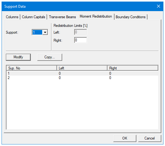
Figure 4-33 Moment Redistribution dialog box
4.7.17Defining Reinforcement Criteria for Slabs and Ribs
In order for spSlab to select the reinforcement, you must define the slab and rib reinforcement, bar sizes, location, and minimum spacing dimensions. See "Area of Reinforcement" and "Reinforcement Selection" in Method of Solution for a discussion of the reinforcement computations.
To define reinforcement Criteria for Slabs and Ribs:
•Select the Reinforcement Criteria command from the Input menu or click the  button on the tool bar. Select Slabs and Ribs tab by clicking the left mouse button on the tab title. The dialog boxes of Figure 4-34 will appear.
•For slabs and ribs, enter the clear covers for top and bottom reinforcing bars. For the top reinforcement, this distance is from the top of the slab to the top of the top bars. For the bottom reinforcement, this distance is from the bottom of the slab to the bottom of the bottom bars (see Figure 4-35). The default value is 1.5 in. [40mm] for both input items.
•Enter the minimum bar size to start the iteration for determining flexural reinforcement.
•Enter the maximum bar size. This number will be used as a stop in the iteration for determining flexural bars in beams.
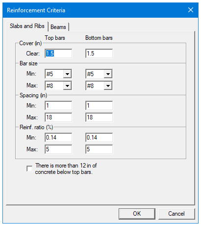
Figure 4-34 Slab and Rib Reinforcement dialog boxes
•Enter minimum bar spacing for slab and rib flexural reinforcement. This number should be based on aggregate size or detailing considerations. Default spacing is 6 in. [150mm] for slabs and ribs.
•Enter maximum bar spacing for slab and rib flexural reinforcement. Default spacing is 18 in. [500 mm] for slabs and ribs.
•Enter minimum Reinforcement Ratio for slab and rib flexural reinforcement. Default ratio is 0.14% [0.20%] for slabs and ribs. If the user specified value is smaller than 0.14%, 0.14% is used by spSlab. If the user specified value is greater than 0.14%, the specified value is used by spSlab.
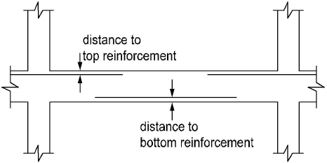
Figure 4-35 Clear Cover to Reinforcement
•Enter maximum Reinforcement Ratio for slab and rib flexural reinforcement. Default ratio is 5% for slabs and ribs.
•If the top bars have more than 12 in. [300 mm] of concrete below them, check the corresponding check box.
•Press Ok button to exit the dialog box and allow spSlab to use the new data.
4.7.18Defining Reinforcement Criteria for Beams
In order for spSlab to select the reinforcement, you must define the beam reinforcement, bar sizes, location, and minimum spacing dimensions. See "Area of Reinforcement" and "Reinforcement Selection" in the Method of Solution for a discussion of the reinforcement computations.
To define reinforcement criteria for beams:
•Select the Reinforcement Criteria command from the Input menu or click the  button on the tool bar. Select Beams tab by clicking the left mouse button on the tab title. The dialog boxes of Figure 4-36 will appear.
•Enter the covers for top and bottom reinforcing bars for beams. For the top reinforcement, this distance is from the top of the beam to the top of the top bars; and for the bottom reinforcement, this distance is from the bottom of the beam to the bottom of the bottom bars (see Figure 4-37). The default value is 1.5 in. [40mm] for both input items.
•Enter the side cover which is measured from the side face of a beam to the face of the stirrup (see Figure 2-20). The default value is 1.5 in [40 mm].
•Enter the minimum bar size for top and bottom bars and stirrups to start the iteration for determining flexural reinforcement.
•Enter the maximum bar size for top and bottom bars and stirrups. This number will be used as a stop in the iteration for determining flexural bars in beams.
•Enter the minimum bar spacing for beam flexural reinforcement and stirrups. This number should be based on aggregate size or detailing considerations. The default minimum reinforcement bar spacing is 1 in. [25 mm] and the default stirrup spacing is 6 in. [150 mm]
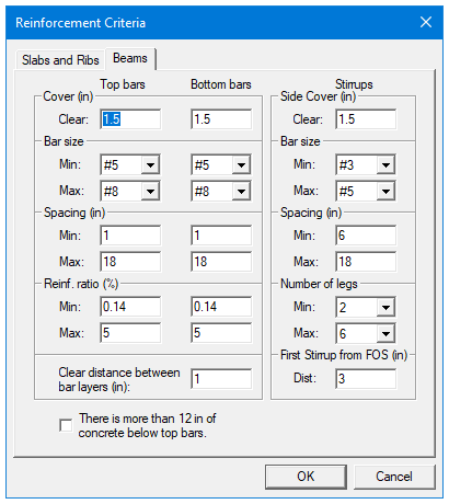
Figure 4-36 Beam reinforcement dialog boxes
•Enter the maximum bar spacing for beam flexural reinforcement and stirrups. The default maximum reinforcement spacing is 18 in. [500 mm] and the default maximum stirrup spacing is 18 in. [450 mm]
•Enter the minimum Reinforcement Ratio for beam flexural reinforcement. Default ratio is 0.14% [0.20%] for beams. If the user specified value is smaller than 0.14%, 0.14% is used by spSlab. If the user specified value is greater than 0.14%, the specified value is used by spSlab.
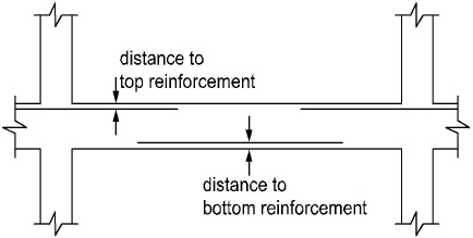
Figure 4-37 Clear Cover to Reinforcement
•Enter the maximum Reinforcement Ratio for beam flexural reinforcement. Default ratio is 5% for beams.
•Enter the clear distance between bar layers to use if the program needs to distribute flexural bars in multiple layers. Default distance is 1 in. [30 mm] for beams.
•Enter the distance from face of support (FOS) to first stirrup. The default value is 3.0 in [75 mm].
•If the top bars have more than 12 in. [300 mm] of concrete below them, check the corresponding check box.
•Press Ok button to exit the dialog box and allow spSlab to use the new data.
4.7.19Defining Column Strip Bars for Two-Way Slab Systems
The reinforcing bar size, number of bars, bar length, etc. can be defined by users if the Run Mode of Investigation and two-way floor system are selected in the General Information dialog box. This menu item is not available if Run Mode of Design is selected in the General Information dialog box.
To define column strip bars:
1.Select Reinforcing Bars from the Input menu or click the  button on the tool bar. Select the Column Strip Bars tab by clicking the tab title or use the tab key on the keyboard to toggle to the tab title then select the Column Strip Bars tab using the arrow keys. The dialog boxes of Figure 4-38 will appear.
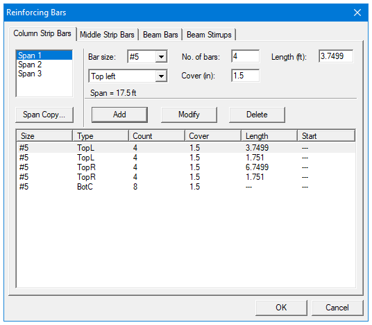
Figure 4-38 Defining Column Strip Bars
2.Select the span for which reinforcing bars will be defined from the Span list box on the upper left corner. The length of the selected span will be shown right above the Add button.
3.Select bar size from the Bar Size drop-down list.
4.Define the number of reinforcing bars in the selected span by entering the number in the Number of Bars input box.
5.Define the length of the reinforcing bars by entering the length in the Length input box. The unit of the length is foot [m].
6.Define the types of the reinforcing bars in the selected span by selecting from the Type drop-down list, which is right below the Bar Size drop-down list. Five types are available: Top Left, Top Right, Top Continuous, Bottom Continuous and Bottom Discontinuous.
7.Define the cover by entering the number in the Cover input box. The unit of cover is inch [mm].
8.Press Add button to add the new data into the list box below the buttons.
9.Repeat steps 2 to 8 to define reinforcing bars for all the spans. You may use the Span Copy button below the Span list to simply copy the data of one span to other spans.
10.If the reinforcing data of a span needs to be modified, select the data from the data list box on the lower part of the dialog box then modify the data as mentioned above. Press Modify button when finished to update the corresponding data in the data list box.
11.To delete the reinforcing data for a span, select the data of the span from the data list box then press the Delete button.
12.Press Ok button to exit the dialog box so that spSlab will use these reinforcing bar properties.
4.7.20Defining Middle Strip Bars for Two-Way Slab Systems
The reinforcing bar size, number of bars, bar length, etc., can be defined by users if the Run Mode of Investigation and two-way floor system are selected in the General Information dialog box. This menu item is not available if Run Mode of Design is selected in the General Information dialog box.
To define middle strip bars:
1.Select Reinforcing Bars from the Input menu or click the  button on the tool bar. Select the Middle Strip Bars tab by clicking the tab title or use the tab key on the keyboard to toggle to the tab title then select the Middle Strip Bars tab using the arrow keys. The dialog boxes of Figure 4-39 will appear.
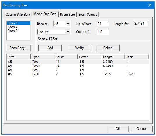
Figure 4-39 Defining Middle Strip Bars
2.Select the span for which reinforcing bars will be defined from the Span list box on the upper left corner. The length of the selected span will be shown right above the Add button.
3.Select bar size from the Bar Size drop-down list.
4.Define the number of reinforcing bars in the selected span by entering the number in the Number of Bars input box.
5.Define the length of the reinforcing bars by entering the length in the Length input box. The unit of the length is foot [m].
6.Define the Types of the reinforcing bars in the selected span by selecting from the drop-down list, which is right below the Bar Size drop-down list. Five types are available: Top Left, Top Right, Top Continuous, Bottom Continuous and Bottom Discontinuous.
7.Define the cover by entering the number in the Cover input box. The unit of cover is inch [mm].
8.Press Add button to add the new data into the list box below the buttons.
9.Repeat steps 2 to 8 to define reinforcing bars for all the spans. You may use the Span Copy button below the Span list to simply copy the data of one span to other spans.
10.If the reinforcing data of a span needs to be modified, select the data from the data list box on the lower part of the dialog box then modify the data as mentioned above. Press Modify button when finished to update the corresponding data in the data list.
11.To delete the reinforcing data for a span, select the data of the span from the data list box then press the Delete button.
12.Press Ok button to exit the dialog box so that spSlab will use these reinforcing bar properties.
4.7.21Defining Beam Bars for Two-Way Slab Systems
The reinforcing bar size, number of bars, bar length, etc. can be defined by users if the Run Mode of Investigation and two-way floor system are selected in the General Information dialog box. This menu item is not available if Run Mode of Design is selected in the General Information dialog box.
To define beam bars:
1.Select Reinforcing Bars from the Input menu or click the  button from the tool bar. Select the Beam Bars tab by clicking the tab title or use the tab key on the keyboard to toggle to the tab title then select the Beam Bars tab using the arrow keys. The dialog box of Figure 4-40 will appear.
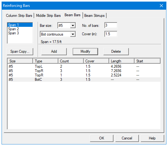
Figure 4-40 Defining Beam Bars
2.Select the span for which reinforcing bars will be defined from the Span list box on the upper left corner. The length of the selected span will be shown right above the Add button.
3.Select bar size from the Bar Size drop-down list.
4.Define the number of reinforcing bars in the selected span by entering the number in the Number of Bars input box.
5.Define the length of the reinforcing bars by entering the length in the Length input box. The unit of the length is foot [m].
6.Define the types of the reinforcing bars in the selected span by selecting from the Type drop-down list, which is right below the Bar Size drop-down list. Five types are available: Top Left, Top Right, Top Continuous, Bottom Continuous and Bottom Discontinuous.
7.Define the cover by entering the number in the Cover input box. The unit of cover is inch [mm].
8.Press Add button to add the new data into the list box below the buttons.
9.Repeat steps 2 to 8 to define reinforcing bars for all the spans. You may use the Span Copy button below the Span list to simply copy the data of one span to other spans.
10.If the reinforcing data of a span needs to be modified, select the data from the data list box on the lower part of the dialog box then modify the data as mentioned above. Press Modify button when finished to update the corresponding data in the data list.
11.To delete the reinforcing data for a span, select the data of the span from the data list box then press the Delete button.
Press Ok button to exit the dialog box so that spSlab will use these reinforcing bar properties.
4.7.22Defining Beam Stirrups for Two-Way Slab Systems
The stirrup size, number of stirrups, etc. can be defined by users if the Run Mode of Investigation and two-way floor system are selected in the General Information dialog box. This menu item is not available if Run Mode of Design is selected in the General Information dialog box.
To define beam stirrups:
1.Select Reinforcing Bars from the Input menu or click the  button from the tool bar. Select the Beam Stirrups tab by clicking the tab title or use the tab key on the keyboard to toggle to the tab title then select the Beam Stirrups tab using the arrow keys. The dialog boxes of Figure 4-41 will appear.
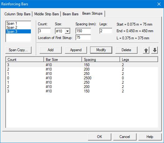
Figure 4-41 Defining Beam Stirrups
2.Select the span for which stirrups will be defined from the Span list box on the upper left corner. The length of the selected span will be shown right above the Add button.
3.Enter the amount of stirrups of the selected span in the Count input box. (see Note)
4.Select stirrup size from the Size drop-down list.
5.Enter the spacing of the stirrups of the selected span in the Spacing input box. The unit of spacing is inch [mm].
6.Enter the number of legs in the Leg input box.
7.For first stirrup set modify the default location of first stirrup if required.
8.Press Add button to add the new data into the list box below the buttons.
9.Repeat steps 2 to 8 to define stirrups for all the spans. You may use the Span Copy button below the Span list to simply copy the data of one span to other spans.
10.In order to mirror stirrup set or sets at the end of the span use Append button.
11.If the stirrup data of a span needs to be modified, select the data from the data list box on the lower part of the dialog box then modify the data as mentioned above. Press Modify button when finished to update the corresponding data in the data list.
12.To delete the stirrup data for a span, select the data of the span from the data list box then press the Delete button.
13.Press Ok button to exit the dialog box so that spSlab will use these reinforcing bar properties.
Note: If stirrups do not apply in a part of a span, the Count should be set to 0 (zero) and the Spacing should be the length of the part of the span where no stirrups are defined. For example, the following configuration shows stirrups in the left and right ends of a span with an empty space (46.0 in. long, no stirrups) in the middle part of the span.
|
Count |
Bar Size |
Spacing |
Legs |
|
32 |
#5 |
4.50 |
2 |
|
0 |
#5 |
46.0 |
2 |
|
32 |
#5 |
4.50 |
2 |
4.7.23Defining Flexure Bars for Beams and One-Way Slab Systems
The reinforcing bar size, number of bars, bar length, etc. for one-way beam systems can be defined by users if the Run Mode of Investigation and beams/one-way slab floor system are selected in the General Information dialog box. This menu item is not available if Run Mode of Design is selected in the General Information dialog box.
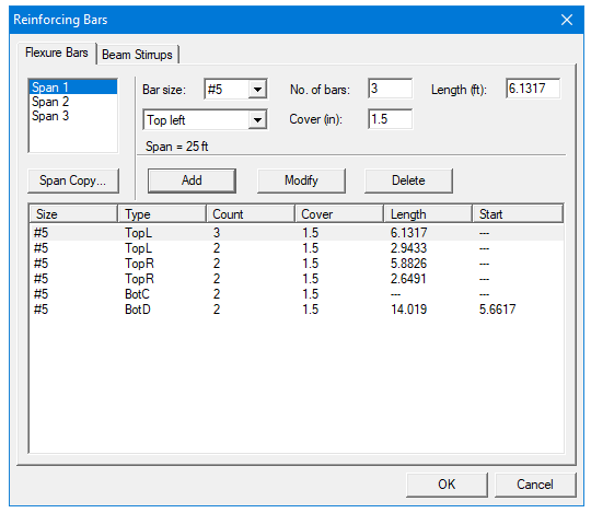
Figure 4-42 Defining Flexure Bars for Beams/One-Way slab Systems
To define flexure bars for beam in beams/one-way slab systems follow the steps described in section Defining Beam Bars.
4.7.24Defining Stirrups for Beams and One-Way Slab Systems
The stirrup size, number of stirrups, etc. for beams/one-way slab systems can be defined by users if the Run Mode of Investigation and beams/one-way slab floor system are selected in the General Information dialog box. This menu item is not available if Run Mode of Design is selected in the General Information dialog box.
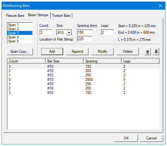
Figure 4-43 Defining Beams Stirrups in Beam/One-Way Slab Systems
To define beam stirrups in beams/one-way slab systems follow the steps described in section Defining Beam Stirrups.
4.7.25Defining Torsional Longitudinal Bars for Beams
The torsional longitudinal reinforcement bars are distributed along the perimeter of the section in addition to the flexure bars. They can be defined by users if the Run Mode of Investigation, beams/one-way slab floor system, and torsional analysis and design are selected in the General Information dialog box. This menu item is not available if Run Mode of Design is selected in the General Information dialog box.
To define torsional longitudinal bars for beams in beams/one-way slab systems:
1.Select Reinforcing Bars from the Input menu or click the  button from the tool bar. Select the Torsion Bars tab by clicking the tab title or use the tab key on the keyboard to toggle to the tab title then select the Torsion Bars tab using the arrow keys. The dialog box of Figure 4-44 will appear.
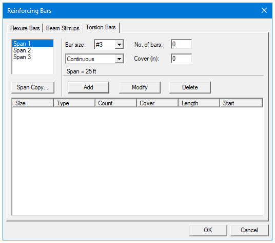
Figure 4-44 Defining Torsion Bars for Beams in Beams/One-Way Slab Systems
2.Select the span for which reinforcing bars will be defined from the Span list box on the upper left corner. The length of the selected span will be shown right above the Add button.
3.Select bar size from the Bar Size drop-down list.
4.Define the type of the reinforcing bars in the selected span by selecting from the Type drop-down list, which is right below the Bar Size drop-down list. Two types are available: Continuous and Discontinuous.
5.Define the number of reinforcing bars in the selected span by entering the number in the Number of Bars input box.
6.Define the cover by entering the number in the Cover input box. The unit of cover is inch [mm].
7.For discontinued bars, define the length and the starting point of the reinforcing bars by entering the values in the Start and Length input boxes. The unit of both is foot [m].
8.Press Add button to add the new data into the list box below the buttons.
9.Repeat steps 2 to 8 to define reinforcing bars for all the spans. You may use the Span Copy button below the Span list to simply copy the data of one span to other spans.
10.If the reinforcing data of a span needs to be modified, select the data from the data list box on the lower part of the dialog box then modify the data as mentioned above. Press Modify button when finished to update the corresponding data in the data list.
11.To delete the reinforcing data for a span, select the data of the span from the data list box then press the Delete button.
12.Press Ok button to exit the dialog box so that spSlab will use these reinforcing bar properties.
Up to 6 load cases of dead load, live load or lateral load can be defined in the Load Cases dialog box. The default five load case labels (types) are SELF (dead load), Dead (dead load), Live (live load), Wind (wind load), and EQ (seismic load).
To define load cases:
1.Select Load Cases command from the Input menu or click the  button on the tool bar. Dialog box as in Figure 4-45 will appear.
2.Enter a name for the new load case in the Label edit box. The name could be any character string defined by the user.
3.Select the type of the new load case from the Type drop-down list. The available types are Dead Load, Live Load and Lateral Load.
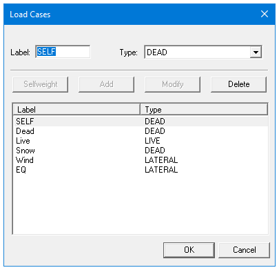
Figure 4-45 Defining Load Cases
4.Press Add button to add the new load case into the load case list box on the lower part of the dialog box.
5.Repeat steps 2 to 4 to define all the load cases. The maximum number of load cases is 6. Once the maximum number is reached, the Add button will be disabled.
6.To enter reserved load case SELF press the Selfweight button.
7.To modify an existing load case, select the load case from the load case list box then change the label or type the selected load case as mentioned above and press the Modify button.
8.To delete an existing load case, select the load case from the load case list box then press the Delete button.
9.Press Ok button to exit the dialog box so that spSlab will use these load cases.
Note: Only one case of live load can be defined. Load case label must be unique for each of the load cases. To ignore self weight in both strength and deflection calculations remove load case SELF from the list of load cases.
4.7.27Defining Load Combinations
spSlab allows you to change the magnification factors applied to the load cases. The default values depend on the code selected with the General Information command.
To define load factors:
1.Select Load Combinations from the Input menu or click the  button from the tool bar. The dialog box of Figure 4-46 will appear if the ACI code was selected in the General Information dialog box.
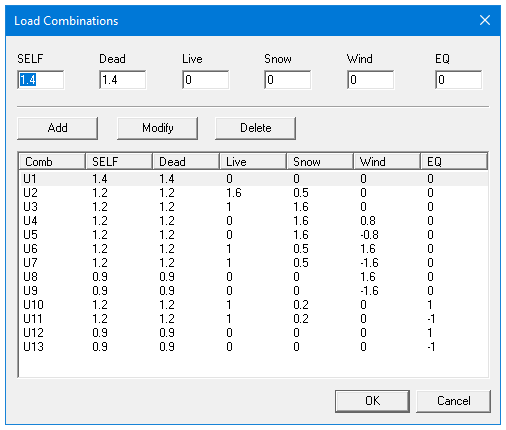
Figure 4-46 Define Load Combinations
2.The load cases and the corresponding factors that are defined in the Load Cases dialog box are shown on the top of the Load Combinations dialog box.
3.Enter the load factors for each of the load cases in the input box below the corresponding load case label.
4.Press the Add button to add the combination defined above into the big list box in the lower part of the dialog box.
5.Repeat steps 2 to 4 to define all the load combinations. Up to fifty load combinations may be defined. All the combinations are indexed automatically from U1 to U50.
6.To change the factors of an existing combination, select the load combination from the load combination list box on the lower part of the dialog box then change the factors as mentioned above. Press the Modify button when finished to update the data in the load combination list box.
7.To delete an existing combination, select the load combination from the load combination list box then press the Delete button.
8.Select Ok button when all the desired load factors have been modified to exit so that spSlab will use the new data.
spSlab computes the self weight of the floor system. Other loads applied to the structure have to be specified by the user. There are several types of applied loads that may be entered. They are found in the Input menu. Surface loads are placed over the entire strip. Partial loads consist of uniform or trapezoidal loads, concentrated loads, and concentrated moments that may exist anywhere within the span length. For beams/one-way slab systems torsional loads can be defined either as concentrated or distributed torques.
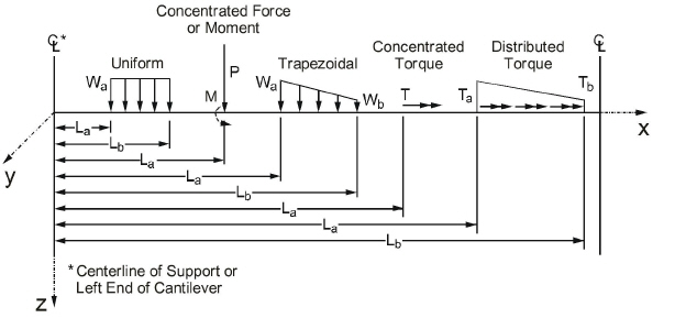
Figure 4-47 Span Load Types
Note: The loads shown in the Figure 4-47 are all positive and may not match the typical sign conventions.
The following table describes input for the span load types shown in Figure 4-48.
|
Wa |
For uniformly distributed loads, Wa is the intensity of the load in units of lbs/ft [kN/m], positive Wa is downward. For trapezoidal loads, Wa is the intensity at the left end in units of lbs/ft [kN/m], positive Wa is downward. For concentrated force, Wa is the force P in units of kips [kN], positive Wa is downward. For concentrated moments, Wa is the moment M in units of ft-kips [kNm], positive Wa is clockwise. For concentrated torque, Wa is the external torque T in units of ft-kips [kNm], positive Wa is such that applying the right hand screw rule the torque vector points to the right. For distributed torque, Wa is the external torque intensity Ta in units of ft-kips/ft [kNm/m], positive Wa is such that applying the right hand screw rule the torque vector points to the right. |
|
Wb |
For trapezoidal loads, Wb is the intensity at the right end in units of lbs/ft [kN/m], positive Wb is downward. For distributed torque, Wb is the external torque intensity Tb in units of ft-kips/ft [kNm/m], positive Wa is such that applying the right hand screw rule the torque vector points to the right. For all the other partial load types, Wb is not available. |
|
La |
For distributed loads, La is the distance where the load begins from the centerline of the column at the left of the span, in units of ft [m]. For concentrated loads and moments, La is the distance where the load exists from the centerline of the column at the left of the span in units of ft [m]. |
|
Lb |
For distributed loads, Lb is the distance where the load ends from the centerline of the column at the left of the span, in units of ft [m]. For concentrated loads and moments, Lb is unavailable. |
4.7.29Defining Area Load on Span
Area loads are uniform loads acting over the entire strip. These loads have units of lb/ft2 [kN/m2].
To input area loads:
1.Select the Span Loads command from the Input menu or click the  button on the tool bar. Select the Area Load from the Type drop-down list on the Span Loads dialog box. The dialog box of Figure 4-48 will appear.
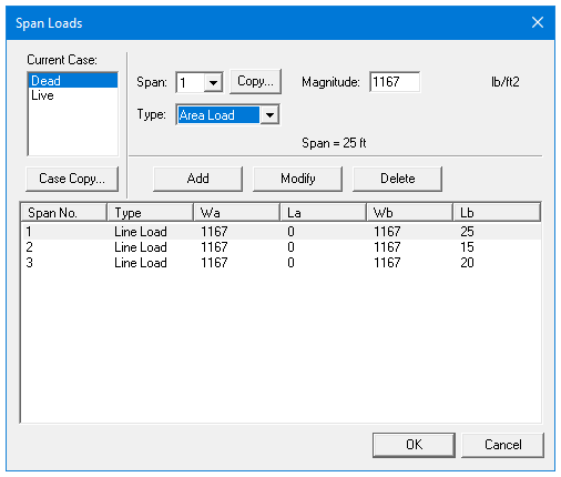
Figure 4-48 Defining Area Load on Span
2.Select the load case from the Current Case list box on the upper left corner as shown in the dialog above.
3.Select the span on which the area loads will be applied from the Span drop-down list.
4.Enter the unfactored superimposed area load magnitude acting over the entire area of the strip in the Magnitude edit box. Positive surface loads act downward.
5.Press the Add button to update the area loads in the area load list box on the lower part of the dialog box.
6.Repeat steps 2 through 5 until the loads have been updated. You can use the Copy button as a shortcut.
7.To change the data of an existing area load, select the area load from the area load list box then change the magnitude as mentioned above. Press the Modify button when finished to update the data in the area load list box.
8.To delete an existing area load, select the load from the area load list box then press the Delete button.
9.Press Ok button to exit the dialog box so that spSlab will use the new data.
4.7.30Defining Line Load on Span
You may enter uniform or trapezoidal loads that do not span from column centerline to column centerline in the direction of analysis. These loads are called line loads and are input through the Span Loads dialog of the Input menu. Partial loads are assumed to act over the entire strip width.
To input line loads:
1.Select the Span Loads command from the Input menu or click the  button on the tool bar. Select the Line Load from the Type drop-down list. The dialog box of Figure 4-49 will appear.
2.Select the load case of the line load that will be defined from the Current Case list box.
3.From the Span drop-down list, select the span number of the span whose line loads you would like to input.
4.Define unfactored load values and their locations in the corresponding text boxes.
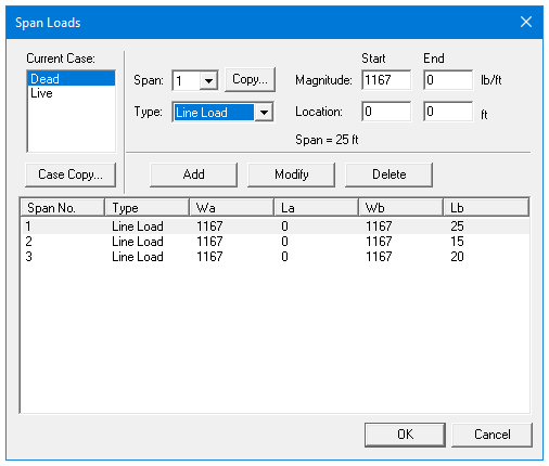
Figure 4-49 Defining Line Load on Span
5.Select Add to add the line load defined into the line load list box.
6.Repeat steps 2 through 5 until all the line loads have been entered then press Ok button to exit the dialog box so that spSlab will use the new loads.
To change line loads data:
•Select the line load you want to change from the line load list box on the lower part of the dialog box by clicking the left mouse button on the load or tabbing to the list box and using the arrow up and down keys.
•Make your changes to the load by modifying the load type, the load magnitude, and/or location.
•Select Modify to replace the old data with the new data.
To delete line load data:
•Select the line load you want to delete from the line load list box by clicking the left mouse button on the load or tabbing to the list box and using the arrow up and down keys.
•Press the Delete button.
4.7.31Defining Point Force on Span
You may enter concentrated vertical loads. These loads are input through the Span Load command of the Input menu. Point loads are assumed to act over the entire strip width.
To input point loads:
1.Select the Span Loads command from the Input menu or click the  button on the tool bar. Select the Point Force from the Type drop-down list. The dialog box of Figure 4-50 will appear.

Figure 4-50 Defining Point Forces on Span
2.Select the load case of the point force that will be defined from the Current Case list box.
3.From the Span drop-down list, select the span number of the span whose point loads you would like to input.
4.Define unfactored load values and their locations in the corresponding text boxes.
5.Select Add to add the point load defined into the point load list box on the lower part of the dialog box.
6.Repeat steps 2 through 5 until all the point loads have been entered then press Ok button to exit the dialog box so that spSlab will use the new loads.
To change point load data:
•Select the point force you want to change from the point load list box by clicking the left mouse button on the load or tabbing to the list box and using the arrow up and down keys.
•Make your changes to the load by modifying the load type, the load magnitude, and/or location.
•Select Modify to replace the old data with the new data.
To delete point load data:
•Select the point force you want to delete from the point load list box to the right by clicking the left mouse button on the load or tabbing to the list box and using the arrow up and down keys.
•Press the Delete button.
4.7.32Defining Point Moment on Span
You may enter concentrated moment. This load is input through the Span Load command of the Input menu. Point moments are assumed to act over the entire strip width.
To input point moments:
1.Select the Span Loads command from the Input menu or click the  button on the tool bar. Select the Point Moment from the Type drop-down list. The dialog box of Figure 4-51 will appear.
2.Select the load case of the point moment that will be defined from the Current Case list box.
3.From the Span drop-down list, select the span number of the span whose point moments you would like to input.
4.Define unfactored moment values and their locations in the corresponding text boxes.
5.Select Add to add the point moment defined into the point moment list box on the lower part of the dialog box.
6.Repeat steps 2 through 5 until all the point moments have been entered then press Ok button to exit the dialog box so that spSlab will use the new moments.

Figure 4-51 Defining Point Moments on Span
To change point moment data:
•Select the point moment you want to change from the point moment list box by clicking the left mouse button on the load or tabbing to the list box and using the arrow up and down keys.
•Make your changes to the moment by modifying the moment type, the moment magnitude, and/or location.
•Select Modify to replace the old data with the new data.
To delete point moment data:
•Select the point moment you want to delete from the point moment list box to the right by clicking the left mouse button on the load or tabbing to the list box and using the arrow up and down keys.
•Press the Delete button.
4.7.33Defining Line Torque on Span
You may enter line torque for beams/one-way slab systems if Torsion Analysis and Design is selected in the General Information dialog box. This load is input through the Span Load command of the Input menu.
To input line torque:
1.Select the Span Loads command from the Input menu or click the  button on the tool bar. Select the Line Torque from the Type drop-down list. The dialog box of Figure 4-52 will appear.
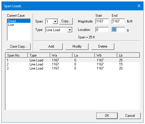
Figure 4-52 Defining Line Torque on Span
2.Select the load case of the line load that will be defined from the Current Case list box.
3.From the Span drop-down list, select the span number of the span whose line loads you would like to input.
4.Define unfactored torque values and their locations in the corresponding text boxes.
5.Select Add to add the line torque defined into the list box.
6.Repeat steps 2 through 5 until all the line torques have been entered. Then press Ok button to exit the dialog box so that spSlab will use the new loads.
To change line torque data:
•Select the line torque you want to change from the load list box on the lower part of the dialog box by clicking the left mouse button on the load or tabbing to the list box and using the arrow up and down keys.
•Make your changes to the load by modifying the load type, the load magnitude, and/or location.
•Select Modify to replace the old data with the new data.
To delete line torque data:
•Select the line torque you want to delete from the load list box by clicking the left mouse button on the load or tabbing to the list box and using the arrow up and down keys.
•Press the Delete button.
4.7.34Defining Point Torque on Span
You may enter point torque for beams/one-way slab systems if Torsion Analysis and Design is selected in the General Information dialog box. This load is input through the Span Load command of the Input menu.
To input point torque:
1.Select the Span Loads command from the Input menu or click the  button on the tool bar. Select the Point Torque from the Type drop-down list. The dialog box of Figure 4-53 will appear.
2.Select the load case of the point torque that will be defined from the Current Case list box.
3.From the Span drop-down list, select the span number of the span whose point moments you would like to input.
4.Define unfactored torque values and their locations in the corresponding text boxes.
5.Select Add to add the point torque defined into the list box on the lower part of the dialog box.
6.Repeat steps 2 through 5 until all the point torques have been entered. Then press Ok button to exit the dialog box so that spSlab will use the new torques.
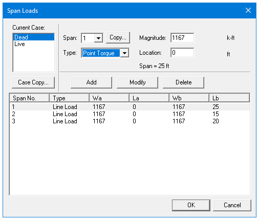
Figure 4-53 Defining Point Torque on Span
To change point torque data:
•Select the point torque you want to change from the list box by clicking the left mouse button on the load or tabbing to the list box and using the arrow up and down keys.
•Make your changes to the moment by modifying the torque magnitude, and/or location.
•Select Modify to replace the old data with the new data.
To delete point torque data:
•Select the point torque you want to delete from the point moment list box by clicking the left mouse button on the load or tabbing to the list box and using the arrow up and down keys.
•Press the Delete button.
4.7.35Defining Support Loads and Displacements
You may enter prescribed support displacements and rotations as well as apply concentrated forces and moments to the system at support locations. These loads are input through the Support Loads and Displacements command of the Input menu.
To input support loads and displacements:
1.Select the Support Loads and Displacements command from the Input menu or click the  button on the tool bar. The dialog box of Figure 4-54 will appear.
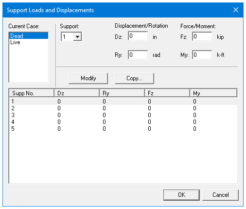
Figure 4-54 Defining Support Loads and Displacements
2.Select the load case of the support loads and displacements that will be defined from the Current Case list box.
3.From the Support drop-down list, select the support number of the support whose loads you would like to input.
4.Define unfactored values of the displacement, rotation, forces, and moment.
5.Select Add to add the support loads and displacements defined into the load list box on the lower part of the dialog box.
6.Repeat steps 2 through 5 until all the support loads and displacements have been entered then press Ok button to exit the dialog box so that spSlab will use the new moments.
To change support and displacement loads data:
•Select the entry you want to change from the load list box by clicking the left mouse button on the load or tabbing to the list box and using the arrow up and down keys.
•Make your changes to the values.
•Select Modify to replace the old data with the new data.
To delete support and displacement load data:
•Select the entry you want to delete from the load list box by clicking the left mouse button on the load or tabbing to the list box and using the arrow up and down keys.
•Press the Delete button.
4.7.36Defining Lateral Effects
spSlab can combine the gravity load analysis with a lateral load analysis. Lateral loads are entered as joint moments obtained elsewhere by a frame analysis. The joint moments are combined with the gravity load moments to produce load patterns 5 through 8.
To input lateral load moments:
1.Define at least one lateral load case from the Load Cases dialog box.
2.Select Lateral Effects from the Input menu. If no lateral case is defined this command is disabled. Once selected, Figure 4-55 will appear.
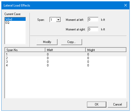
Figure 4-55 Lateral Moment dialog box
3.Select load cases from the Current Case list box. At least one lateral load case must be defined in the Load Cases dialog box before you can see the load case in the Current Case list box.
4.Select span number on which lateral loads will be defined from the Span drop-down list.
5.Enter the moments at the left end and right end of the span in the Moment at Left and Moment at Right input boxes, respectively.
6.Press the Add button to add the lateral load defined above into the lateral load list box in the lower part of the dialog box.
7.Repeat steps 2 through 5 to define all the lateral loads.
8.To change an existing lateral load, select the load from the lateral load list box then change the moments as mentioned above. Press the Modify button when finished to update the data in the lateral load list box.
9.To delete an existing lateral load, select the load from the lateral load list box then press the Delete button.
10.Select Ok button when all the desired lateral loads have been modified to exit so that spSlab will use the new data.
4.8Executing Calculations (menu Solve)
The Execute command starts the design portion of spSlab after you have finished inputting all the data.
To design the system:
Select the Execute command from the Solve menu or click the  button on the tool bar. If any data required to analyze and design the system has not been input prior to executing this command, spSlab will display an "Invalid model!" message. You must complete the data before execution.
An analysis status window shows the current state of the execution as shown in Figure 4-56. If the state of each of the computations is OK, the analysis is successful. If any error is encountered ERROR will be shown and the computation is terminated.

Figure 4-56 Analysis Status Window
Once the analysis and/or design is performed, you can view the results, shear and moment diagrams, and deflected shapes. This section provides procedures performing these functions.
To view the analysis and design results:
•Select Results command from the Solve menu or click the  button from the tool bar. Alternatively you can also press the F6 key. This will launch the spResults module.
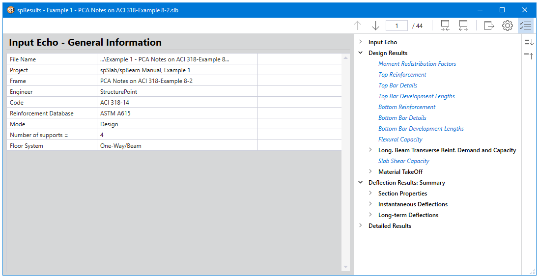
Figure 4-57 spResults Module
•Select the results tables you want to view from the explorer. The table displayed in the preview space will be changed based on your selection.
•To copy results, select desired data from the table and right click, press the Copy button to copy the current results into the Windows clipboard. Then you may use CTRL + V to paste the contents of the clipboard to any other editors such as Word or Notepad.
•Press the Close on the top right corner to close the result dialog box.
4.9View Program Output (menu View)
4.9.1Zooming in on Floor System
In order to view the floor system in greater detail, spSlab allows you to magnify a portion of the floor system for closer analysis.
Using zoom with a magnifier:
•Select Zoom from the View menu then a sub menu appears beside the View menu.
•Select Window from the sub menu. Notice that the Window command is checked and the cursor is changed to a magnifier. The other way to magnify window is to click the  button on the tool bar.
•Move the cross cursor to the upper left corner of the portion of the system you want to enlarge.
•Press and hold down the left mouse button while dragging the cursor to the lower right portion of the system enclosing the desired area within the dashed box.
•Release the mouse to enlarge that portion.
Using Zoom In and Zoom Out command:
•Select Zoom from the View menu and a sub menu appears.
•Select the In(2x) menu command from the sub menu. The current active window will be magnified by two times. The other way to do this is to click the  button on the tool bar.
•Select the Out(0.5x) menu command from the sub menu. The current active window will be reduced by two times. The other way to do this is to click the  button on the tool bar.
Note: To return to original (default) zoom, select Restore from the View menu, or select  from tool bar. To move model in a view window, use Pan from the View menu, or select
  from tool bar.
4.9.2Change Isometric View Angle
You can modify the X and Z angles at which the floor system is displayed in the isometric view window. By default, the floor system is viewed at -45° about the X axis and 45° about the Z axis. The right hand rule is used to determine the angle of rotation about the X and Z axes and the X axis is always rotated first.
To change angles:
•Select Change View Angle from the View menu. The dialog box of Figure 4-58 appears displaying the currently set angles.
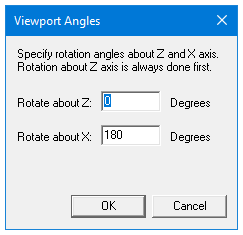
Figure 4-58 Isometric View dialog box
•Change the angles of rotation about the X and Z axes. The X axis is rotated first then the Z axis is rotated. The floor system is rotated about the axis using the right hand rule.
•Select Ok button to accept the new angles and to modify the isometric view.
Note: A more convenient way to change the view angles instantly without entering angles in the dialog box is to use the keyboard shortcut CTRL + ARROW Keys. For example, press CTRL + and CTRL + to rotate the floor system around Z axis and press CTRL + or CTRL + to rotate around X axis.
4.9.3Viewing Specific Member Type
In order to see the floor system members in greater detail, you can select specific member types to view by enabling and disabling them.
To select member type:
•Select the View Options command from the View menu. The dialog box of Figure 4-62 will appear showing the currently displayed member types. Depending on the floor system, some of the member types will be shaded gray and unavailable.
•To hide a member type from a view of the floor system you must remove the P sign from the check box. Click the left mouse button on the check box of the member type you would like to hide. To view a previously hidden member type, click the left mouse button on the check box to add the P sign to the check box.
•Select Ok button to view only the selected member types.
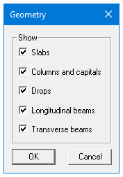
Figure 4-59 View Options dialog box
To switch to plan view:
1.Select the Plan View command from the View menu or click  button on the tool bar. The dialog box of Figure 4-60 will appear.
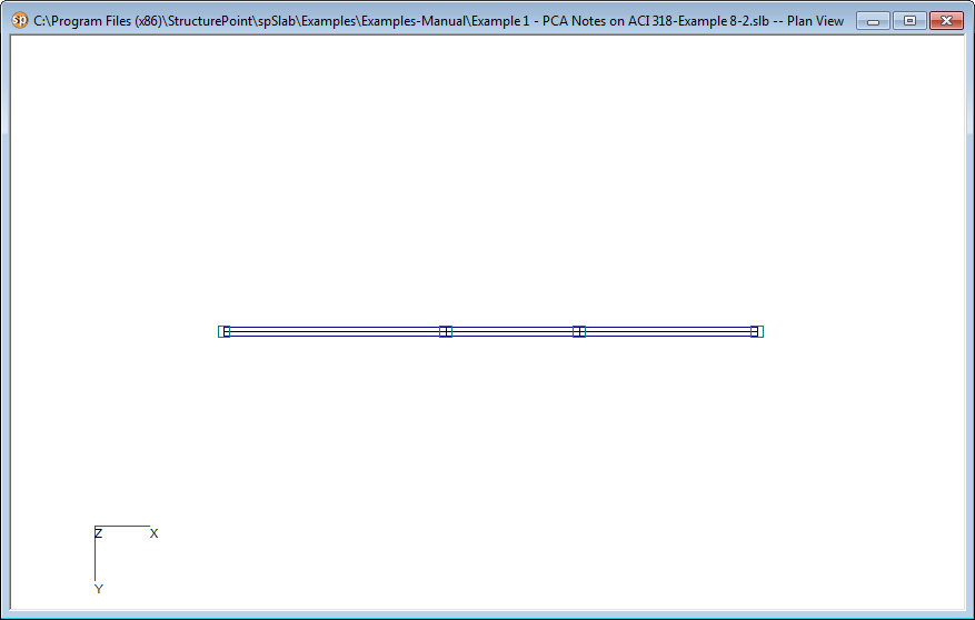
Figure 4-60 Plan View Window
2.Right click on the view window to show the pop-up menu. You may save the current view window as bitmap (BMP) file or metafile (EMF) onto the Windows clipboard by selecting Copy Bitmap or Copy Metafile, respectively. You may also select the commands from the pop-up menu to zoom in or zoom out the view window and preview it before printing it out.

Figure 4-61 Pop-up Menu of View Window
1.Select the Options command from the pop-up menu, and then you may decide what geometry members need to be shown on the view window as shown in Figure 4-62. To hide a member type from a view of the floor system you must remove the P sign from the check box. Click the left mouse button on the check box of the member type you would like to hide. To view a previously hidden member type, click the left mouse button on the check box to add the P sign to the check box.
2.Select Ok button to view only the selected member types.
Figure 4-62 Geometry Options of Elevated View
To switch to elevated view:
•Select the Elevated View command from the View menu or click  button from the tool bar. The dialog box of Figure 4-63 will appear.
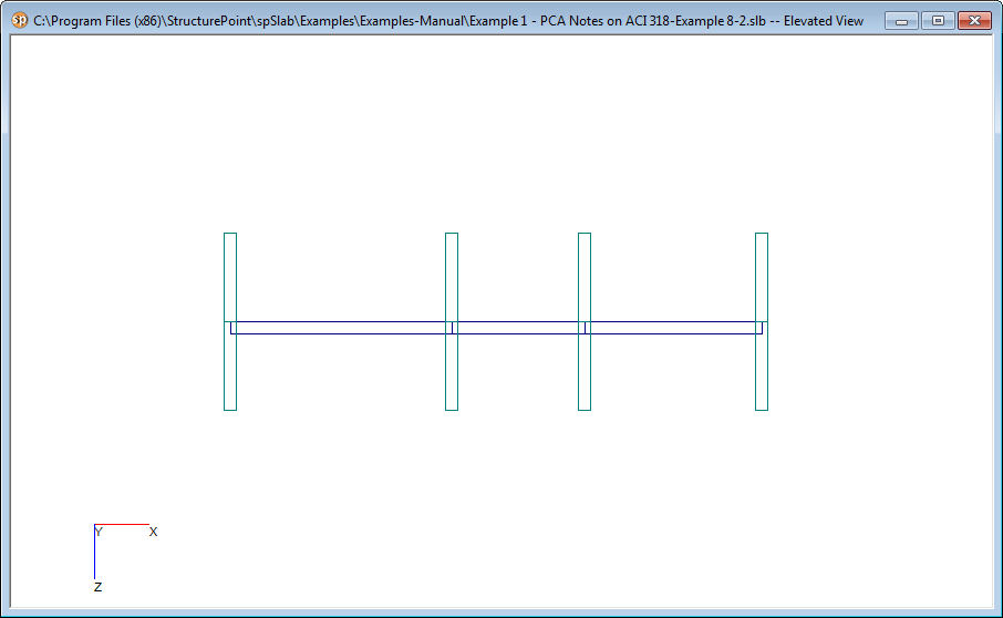
Figure 4-63 Elevated View Window
•Right click on the view window to show the pop-up menu. You may save the current view window as bitmap (BMP) file or metafile (EMF) onto the Windows clipboard by selecting Copy Bitmap or Copy Metafile, respectively. You may also select the commands from the pop-up menu to zoom in or zoom out the view window and preview it before printing it out.
Figure 4-64 Pop-up Menu of View Window
•Select the Options command from the pop-up menu, and then you may decide what geometry members need to be shown on the view window as shown in Figure 4-65. To hide a member type from a view of the floor system you must remove the P sign from the check box. Click the left mouse button on the check box of the member type you would like to hide. To view a previously hidden member type, click the left mouse button on the check box to add the P sign to the check box.
•Select Ok button to view only the selected member types.
Figure 4-65 Geometry Options of Elevated View
To switch to side view:
•Select the Elevated View command from the View menu or click  button from the tool bar. The dialog box of Figure 4-66 will appear.
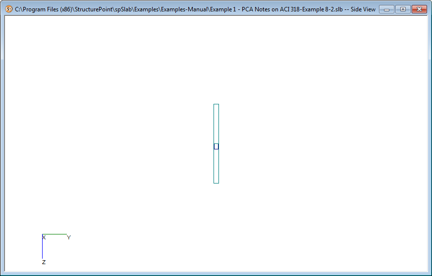
Figure 4-66 Side View window
•Right click on the view window to show the pop-up menu. You may save the current view window as bitmap (BMP) file or metafile (EMF) onto the Windows clipboard by selecting Copy Bitmap or Copy Metafile, respectively. You may also select the commands from the pop-up menu to zoom in or zoom out the view window and preview it before printing it out.
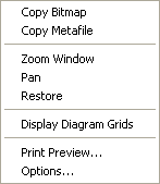
Figure 4-67 Pop-up Menu of View Window
•Select the Options command from the pop-up menu, and then you may decide what geometry members need to be shown on the view window as shown in Figure 4-68. To hide a member type from a view of the floor system you must remove the P sign from the check box. Click the left mouse button on the check box of the member type you would like to hide. To view a previously hidden member type, click the left mouse button on the check box to add the P sign to the check box.
Figure 4-68 Geometry Options of Side View
•Select Ok button to view only the selected member types.
To switch to isometric view:
•Select the Isometric View command from the View menu or click  button on the tool bar. The dialog box of Figure 4-69 will appear.
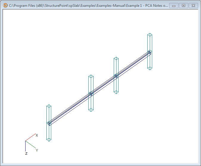
Figure 4-69 Isometric View Window
•Right click on the view window to show the pop-up menu. You may save the current view window as bitmap (BMP) file or metafile (EMF) onto the Windows clipboard by selecting Copy Bitmap or Copy Metafile, respectively. You may also select the commands from the pop-up menu to zoom in or zoom out the view window and preview it before printing it out.

Figure 4-70 Pop-up Menu of View Window
•Select the Options command from the pop-up menu, and then you may decide what geometry members need to be shown on the view window as shown in Figure4-71. To hide a member type from a view of the floor system you must remove the P sign from the check box. Click the left mouse button on the check box of the member type you would like to hide. To view a previously hidden member type, click the left mouse button on the check box to add the P sign to the check box.
Figure 4-71 Geometry Options of Isometric View
•Select Ok button to view only the selected member types.
To show the loads:
•Select the Loads command from the View menu or click  button from the tool bar. The dialog box of Figure 4-72 will appear.
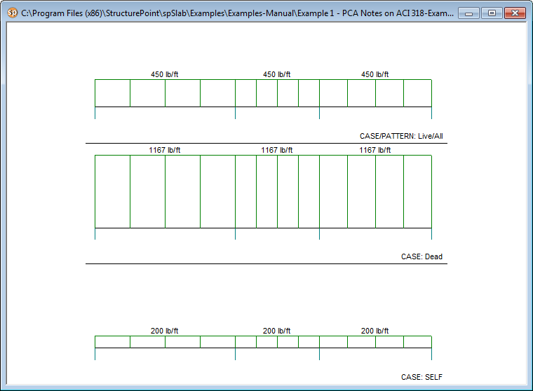
Figure 4-72 Loads View Window
•Right click on the view window to show the pop-up menu. You may save the current view window as bitmap (BMP) file or metafile (EMF) onto the Windows clipboard by selecting Copy Bitmap or Copy Metafile, respectively. You may also select the commands from the pop-up menu to zoom in or zoom out the view window and preview it before printing it out.

Figure 4-73 Pop-up menu of View Window
•Select the Options command from the pop-up menu, and then you may decide what kind of loads need to be shown on the view window as shown in Figure 4-74. To hide a load case, load type, or live load pattern you must remove the P sign from the check box. Click the left mouse button on the check box of the member type you would like to hide. To view a previously hidden load type, click the left mouse button on the check box to add the P sign to the check box.
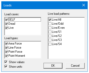
Figure 4-74 Loads Options
•If you want to hide the load values, remove the P sign before Show values check box.
•If you want to hide the load units, remove the P sign before Show units check box.
•Select Ok button to view only the selected member types.
4.9.9.1Viewing Internal Forces Diagrams
Once the design has been performed, you may view the shear, moment, and internal torque (beams/one-way slab systems with torsion) diagrams for any span at any available load combination.
To view shears and moments diagram:
•Select the Internal Forces command from the View menu or click the  button on the tool bar. A view window similar to Figure 4-75 will appear. The upper half view window shows the shear diagram and the lower half the view window shows the moment diagram. If torsion is enabled for beams/one-way slab systems than internal torque diagram will also be shown in this window.
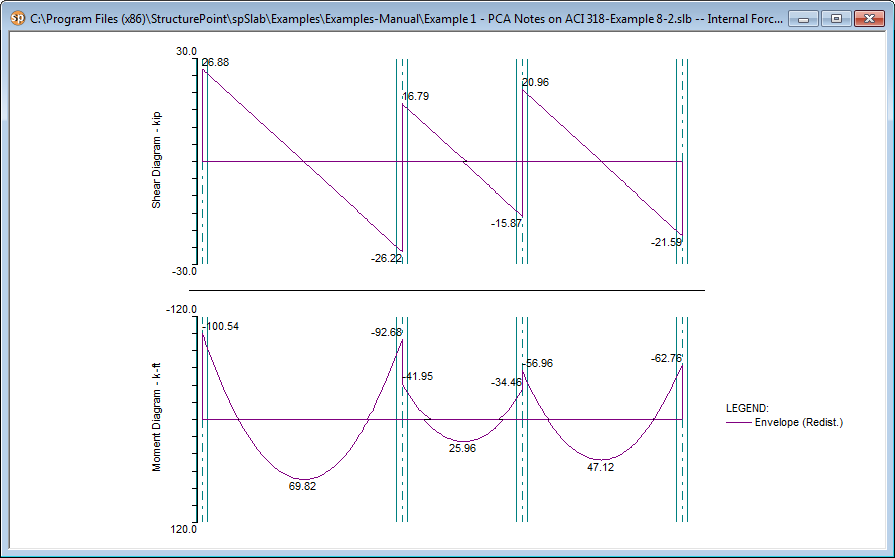
Figure 4-75 View Internal Forces Diagram
•The current coordinate values can be captured based on the position of the mouse cursor. The status bar in Figure 4-76 shows the name of the diagram, two coordinate values of the current mouse cursor position, and the current design code used in the project.

Figure 4-76 Coordinate Value Shown in Status Bar
•Click the right mouse button anywhere on the view window to show the pop-up menu. You may Restore, Zoom, Pan or Print View directly by selecting commands from this pop-up menu.
•Click the Options command from the pop-up menu to change the span for which the internal forces diagrams will be shown and to choose if legend will be displayed or not. Figure 4-77 shows the Options dialog box. Select a span number from the Show diagram for drop-down list and select a load Envelope or combination from the Select load combinations check list box. Use Draw Legend checkbox to control whether legend is drawn or not. Press the Ok button to close the dialog box and redraw the view windows.
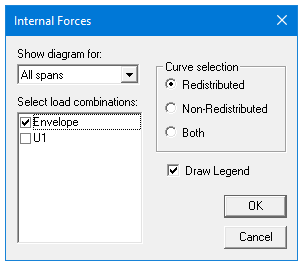
Figure 4-77 View Internal Forces Diagram Options
Note: The pop-up menu can be accessed from each of the view windows of spSlab.
The Restore command cannot be executed in the pop-up menu until the Zoom or Pan command is stopped by pressing the ESC key. Without stopping the Zoom/Pan command, one can only restore a view using the Restore command in View menu or  button in the tool bar. This occurs in all spSlab view windows.
4.9.9.2Viewing Moment Capacity
Once the design has been performed, you may view the moment capacity diagrams for any span. The moment capacity window will be split in half horizontally. The middle strip moment capacity will occupy the upper half and the column strip moment capacity will occupy the lower half where each diagram will be scaled to fill the entire half of the window.
To view moment capacity:
1.Select the Moment Capacity command from the View menu or click the  button on the tool bar. A view window similar to Figure 4-78 will appear.
2.Right click on the Moment Capacity view window and select Options command from the pop-up menu. A dialog box similar to Figure 4-79 will appear.
3.The current coordinate values can be captured based on the position of the mouse cursor. The status bar shows the name of the diagram, two coordinate values of the current mouse cursor position, and the current design code used in the project.
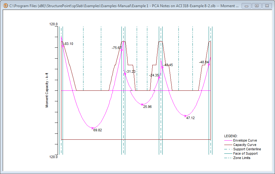
Figure 4-78 View Moment Capacity Diagram
4.Click the right mouse button anywhere on the view window to show the pop-up menu. You may Restore, Zoom, Pan or Print View directly by selecting commands from this pop-up menu.
5.Click the Options command from the pop-up menu to change the span for which the moment capacity will be shown. Select which span will be shown in the Show diagram for drop-down list. Use Draw Legend checkbox to control whether legend is drawn or not. Use VALUES AND ZONES checkbox to control whether values at critical sections within the zones are drawn or not.Select which part of the selected span will be shown in the Show frame box.
To view capacity of longitudinal reinforcement, use Combined M-V-T checkbox (Figure 4-79b) for beams designed or investigated per CSA A23.3-14/042 with Combined M-V-T option.
6.Press the Ok button to close the dialog box and redraw the view windows.
7.The magnitude of the bending moment at the critical sections is displayed and indicated by an asterisk where the bending moment diagram intersects the critical section.
a) 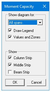 b)
b) 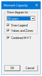
Figure 4-79 View Moment Capacity Option dialog box (a) two-way system (b) beam with M-V-T option selected in Solve Options (CSA A23.3-14/04 only)
Once the design has been performed, you may view the slab shear capacity diagrams for any span.
To view shear capacity:
1.Select the Shear Capacity command from the View menu or click the  button on the tool bar. A view window similar to Figure 4-80 will appear.
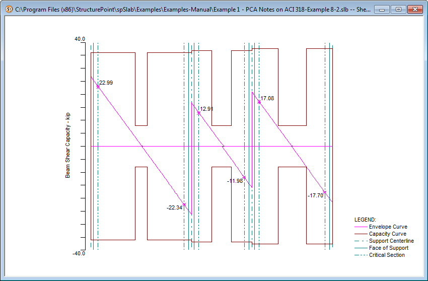
Figure 4-80 View Shear Capacity
•Right click on the Shear Capacity view window and select Options command from the pop-up menu. A dialog box similar to Figure 4-81 will appear.
a) 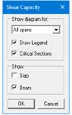 b)
b) 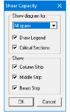
Figure 4-81 View Shear Capacity Option dialog box(a) One-way and two-way system (b) Two-way system with shear distributed to slab strips
•The current coordinate values can be captured based on the position of the mouse cursor. The status bar shows the name of the diagram, two coordinate values of the current mouse cursor position, and the current design code used in the project.
•Click the right mouse button anywhere on the view window to show the pop-up menu. You may Restore, Zoom, Pan or Print View directly by selecting commands from this pop-up menu.
•Click the Options command from the pop-up menu to change the span for which the shear capacity will be shown. Select which span will be shown in the Show diagram for drop-down list. Use Draw Legend checkbox and Critical Section checkbox to control if the legend and critical sections are drawn or not. Select which part of the selected span will be shown in the Show frame box.
•The magnitude of the shear at critical sections is displayed and indicated by an asterisk where the shear force diagram intersects the critical section.
•Press the Ok button to close the dialog box and redraw the view windows.
Once the design has been performed, you may view the reinforcement diagrams for any span. The reinforcement window will be split in half horizontally. The middle strip reinforcement will occupy the upper half, and the column strip reinforcement will occupy the lower half where each diagram will be scaled to fill the entire half of the window.
To view reinforcement:
•Select the Reinforcement command from the View menu or click the  button on the tool bar. A view window similar to Figure 4-82 will appear.
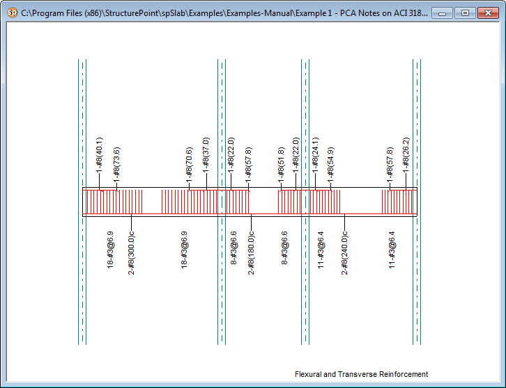
Figure 4-82 View Reinforcement
•Right click on the Reinforcements view window and select Options command from the pop-up menu. A dialog box similar to Figure 4-83 will appear.
•The current coordinate values can be captured based on the position of the mouse cursor. The status bar shows the name of the diagram, coordinate value of the current mouse cursor position in the design direction, and the current design code used in the project.
•Click the right mouse button anywhere on the view window to show the pop-up menu. You may Restore, Zoom, Pan or Print View directly by selecting commands from this pop-up menu.
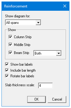
Figure 4-83 View Reinforcement Options dialog box
•Click the Options command from the pop-up menu to change the span for which the shear capacity will be shown. Select the span you want to show from the Show diagram for drop-down list. Select which part of the selected span will be shown from the Show frame box. Checking the Show bar Labels will show labels beside each reinforcement on the view. Similarly bar length can be included by checking Include Bar Length. Bar labels can also be arranged vertically if Rotate Bar Labels is checked. Set the vertical scale (relative to the horizontal scale which is set automatically) to which members are drawn in the Slab Thickness Scale edit box.
•Press the Ok button to close the dialog box and redraw the view windows.
4.9.9.5Viewing Deflected Shapes
Once the design has been performed, you may view the deflection shapes for any span.
To view the deflection shapes:
•Select the Deflection command from the View menu or click the  button on the tool bar. A view window similar to Figure 4-84 will appear.
•Right click on the deflection view window and select Options command from the pop-up menu. A dialog box similar to Figure 4-85 will appear.
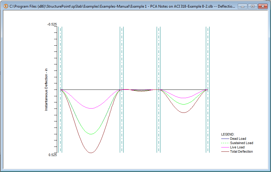
Figure 4-84 View Deflection Diagram
•The current coordinate values can be captured based on the position of the mouse cursor. The status bar shows the name of the diagram, two coordinate values of the current mouse cursor position, and the current design code used in the project.
•Click the right mouse button anywhere on the view window to show the pop-up menu. You may Restore, Zoom, Pan or Print View directly by selecting commands from this pop-up menu.
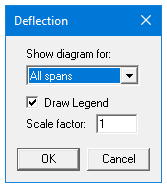
Figure 4-85 View Deflection Option dialog box
•Click the Options command from the pop-up menu to change the span for which the deflection will be shown. Select the span you want to show from the Show Diagram For drop-down list. Check the Draw Legend checkbox to include the legend in the drawing. Enter the scale factor in the Scale Factor edit box. The bigger the scale factor, the more apparent the deflections will be on the diagram.
•Press the Ok button to close the dialog box and redraw the view windows.
4.9.10.1Printing Analysis and Design Results
Once the analysis and/or design is performed, you can print the results. This section provides procedures for performing these functions.
To print the analysis and design results:
Select Reporter command from the Solve menu or click the  button from the tool bar. Alternatively you can also press the F7 key. This will launch the spReporter module.
Figure 4-86 View and Print dialog box
•Only Word/PDF and Text reports can be previewed and directly printed. Select the format you want to print the results in from the panel on the left. The preview will be changed depending on your selection.
•You can adjust the paper size, page orientation margins and print range using the Print/Export panel on the left.
•Press the Print button on the dialog box to print the results through a printer. The printer could be a local printer which is connected to your computer directly, or a network printer.
•Press the Close button to close spReporter when printing job is done.
4.9.10.2Printing Current View Window
Once the design has been performed, you may print the diagrams and views for any span at any available loading pattern by selecting the Print View command from the File menu.
To print a displaying window:
•To select the diagram or view you want to print, single click the left mouse button on the diagram or view window.
•Select the Print View command from the File menu. A print preview window similar to Figure 4-87 will be shown
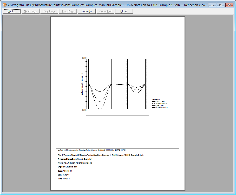
Figure 4-87 Print Preview Window
•Press the Zoom In or Zoom Out buttons or simply click the left mouse button on the preview to magnify or reduce the size of the preview paper.
•Press the Next Page button if more than one page need to be printed.
•Press the Print button to print the view. The printer could be a local printer which is connected to your computer directly, or a network printer.
•Press the Close button to close the preview window and go back to spSlab.
The Print Preview command allows you to preview and print the current view window (floor system geometry in the plan, elevated and isometric views, prints the shear and moment diagrams, and the deflected shapes).
•To obtain a view window you must first perform the design, then select what you want to view from the View menu. You may have more than one view window opened. The current view window is the one activated and on top of the others on your screen.
•Selecting this command closes the spSlab main window and opens the print preview window as shown in Figure 4-87.
•On the print preview window, press the Zoom In or Zoom Out buttons or simply click the left mouse button on the preview window to magnify or reduce the size of the preview paper.
•Press the Next Page button if more than one page needs to be printed.
•Press the Print button to print the view. The printer could be a local printer which is connected to your computer directly, or a network printer.
•Press the Close button to close the preview window and go back to spSlab.
4.9.12Copy Graphs to Clipboard
Copy Bitmap (BMP format)
spSlab can copy any of the ten view windows onto Windows clipboard as bitmap. The bitmap on clipboard can then be pasted into Microsoft Word or other Windows applications including presentation software such as Microsoft PowerPoint.
To copy view window to clipboard as bitmap:
•Select the view window that will be copied by single clicking left mouse button on it.
•Select  from the tool bar to copy the selected view window to clipboard.
•Switch to other word processing software, such as Microsoft Word, then press the CTRL + V to paste the bitmap on clipboard to a Word file.
Copy Metafile (EMF format)
Since bitmap files cannot easily be resized or re-proportioned without significant distortion to the image, metafiles are generally used for situations requiring scalability of the image.
Advantages of metafiles are:
•Large, simply structured images require less memory than bitmaps for display and make optimal use of the resolution of the output device.
•Metafiles can be resized with none of the distortion which normally accompanies resizing of bitmaps.
•A metafile can contain SelectPalette statements, allowing custom palettes to be displayed in applications such as Microsoft Word.
The Enhanced MetaFile (EMF) format is an extension of the Windows metafiles format developed for use with 32 bit Windows applications. It is only available to native 32 bit applications.
To copy view window to clipboard as Enhanced MetaFile (EMF):
•Select the view window that will be copied by single clicking left mouse button on it.
•Select  from the tool bar to copy the selected view window to clipboard.
•Switch to other word processing software, such as Microsoft Word, then press the CTRL + V to paste the bitmap on clipboard to a Word file.
4.10Customizing Program (menu Options)
Colors can be changed for background of views, geometry items such as slabs and beams, text on views, result diagrams, etc.
To change colors:
•Select Colors command from the Options menu. Figure 4-88 will appear.
•From the General frame box on the left side, select the item whose color needs to be changed from the list box.
•Select a color from the Change color to drop-down list. Once a new color is selected from the drop-down list the color in the list box above the drop-down list is updated instantly.
•From the Results category box on the right side, select the item whose color needs to be changed from the list box.
•Select a color from the Change color to drop-down list. Once a new color is selected from the drop-down list the color in the list box above the drop-down list is updated instantly.
•If you want to print views in black and white, select the Print Black and White check box.
•If you want to save the settings as default, select the Save setting for future use check box.
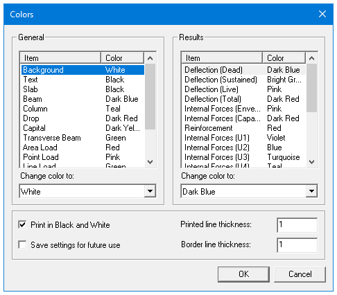
Figure 4-88 Changing Colors dialog box
•Input the line thickness in the Printed Line Thickness edit box. The diagram line thickness will be based on the number you input.
•Press the Ok button to save the settings and close the dialog box.
Fonts can be selected separately for graphical on screen, graphical output and the text output via Options|Font command.
To change the graphical on screen or graphical output fonts:
•Select the Font|Graphical, On Screen or Font|Graphical, Output command from the Options menu. A view window similar to Figure 4-89 will appear.
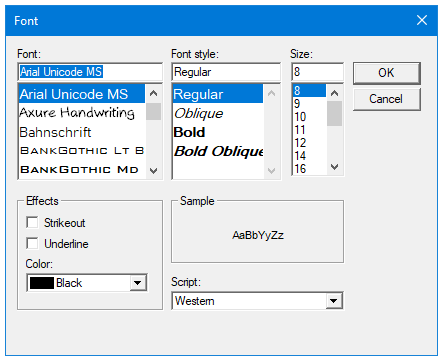
Figure 4-89 Changing Graphical Output Font dialog box
•Select the font, font style and size from the lists. Font sizes different from those on the list can be typed in the Size text box.
•In the Effect frame select if strikeout and/or underline effect have to be applied. Alternatively to the Color dialog box, the font color can be chosen in this dialog box too.
•The script of the font by default is Western and should not be changed.
•Press the Ok button to save the new setting and close the dialog box.
To change the text output font follow the same procedure as for the graphical output font except that font effects are not available for text output and the list of fonts only contains non-proportional fonts which are suitable for tabulated text output (Figure 4-90).
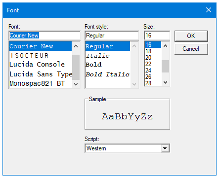
Figure 4-90 Changing Text Output Font dialog box
4.11Working with View Windows (menu Window)
Cascade
The Cascade command displays all the open windows in the same size, arranging them on top of each other so that the title bar of each is visible. The current active view widow will be on the top after the execution of the Cascade command.
Tile Horizontal
The Tile Horizontal command arranges all open windows horizontally so that no window overlaps another. The current active view widow will be on the most left or on the upper-left corner of the screen after the execution of the Tile Horizontal command.
Tile Vertical
The Tile Vertical command arranges all open windows vertically so that no window overlaps another. The current active view widow will be on the most left or on the upper-left corner of the screen after the execution of the Tile Vertical command.
Remaining Commands
The remaining menu items are in a list of the windows that are available for viewing. Selecting any window from this menu will restore the window to its previous size and position from an icon.
4.12Obtaining Help Information (menu Help)
4.12.1Opening Table of Contents of the Help System
To open table of contents of the Help system:
•Select Help from the Help menu.
•Select the chapter you need from the content tree view in the left pane of the browser window. The contents of the selected chapter appear in the right pane of the browser window.
To display the manual:
•Select Manual from the Help menu.
•The manual will be displayed in the default browser window.
To check if a newer version of the program is available:
•Select Check for Updates from the Help menu.
•The program will open the default browser window with the page where the newer version can be requested or downloaded.
4.12.4Obtaining Information about the Program
The following information about the program is displayed in the About spSlab dialog box:
•program version and short description
•licensing information
•the copyright information
The licensing information depends on the type of license being used. If it is a trial license then the License Exp field shows when the trial period expires and the Locking Code field displays a unique fingerprint of the computer on which the program is running. This locking code needs to be provided to StructurePoint in order to generate a permanent license. For other, non-trial licenses, license ID is displayed. You may be asked to provide this ID when you contact StructurePoint for technical support.
To obtain the information about the program:
•Select the About spSlab command from the Help menu. A dialog box of Figure 4-91 will appear.
•Press Ok button to exit the dialog box.
a) 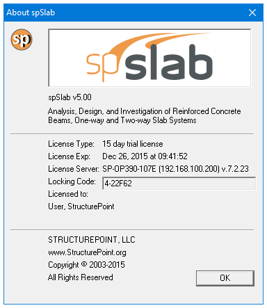 b)
b) 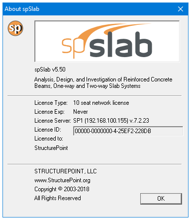
Figure 4-91 About spSlab dialog boxes with (a) a trial license (b) a network license